Improving language models by retrieving from trillions of tokens
arXiv:2112.04426v3 · This workspace stays on this version. Check arXiv for newer versions
Some source details need review 2 to check
Original formulas, table values and figures are preserved. Comparison can miss differences; use the original PDF to check details.
Reading view checked: 600 math expressions, 90 rendering failures; 33 of 33 images available.
Compared 131 of 145 source passages against 37 of 43 PDF pages.
The HTML source contains failed formatting commands; these were omitted from the reading view. The original sources are retained. (2)
- Some formulas could not be rendered; their original TeX is shown. Check the original PDF. (90)
- This long paper was only partially compared; the original sources remain available.
33 of 33 figure, table and graphic images captured. Open original PDF
Abstract
We enhance auto-regressive language models by conditioning on document chunks retrieved from a large corpus, based on local similarity with preceding tokens. With a 2 trillion token database, our Retrieval-Enhanced Transformer (Retro) obtains comparable performance to GPT-3 and Jurassic-1 on the Pile, despite using 25 fewer parameters. After fine-tuning, Retro performance translates to downstream knowledge-intensive tasks such as question answering. Retro combines a frozen Bert retriever, a differentiable encoder and a chunked cross-attention mechanism to predict tokens based on an order of magnitude more data than what is typically consumed during training. We typically train Retro from scratch, yet can also rapidly Retrofit pre-trained transformers with retrieval and still achieve good performance. Our work opens up new avenues for improving language models through explicit memory at unprecedented scale.
Language modelling (LM) is an unsupervised task that consists of modelling the probability of text, usually by factorising it into conditional next-token predictions . Neural networks have proven to be powerful language models, first in the form of recurrent architectures (Mikolov et al., 2010; Graves, 2013; Jozefowicz et al., 2016) and more recently in the form of Transformers (Vaswani et al., 2017), that use attention to contextualise the past. Large performance improvements have come from increasing the amount of data, training compute, or model parameters. Transformers have been scaled from million parameter models in seminal work to over hundred billion parameters (Radford et al., 2019; Brown et al., 2020) in the last two years which has led to models that do very well on a wide array of tasks in a zero or few-shot formulation. Increasing model size predictably improves performance on a wide range of downstream tasks (Kaplan et al., 2020). The benefits of increasing the number of parameters come from two factors: additional computations at training and inference time, and increased memorization of the training data.
In this work, we endeavor to decouple these, by exploring efficient means of augmenting language models with a massive-scale memory without significantly increasing computations. Specifically, we suggest retrieval from a large text database as a complementary path to scaling language models. Instead of increasing the size of the model and training on more data, we equip models with the ability to directly access a large database to perform predictions—a semi-parametric approach. At a high level, our Retrieval Transformer (Retro) model splits the input sequence into chunks and retrieves text similar to the previous chunk to improve the predictions in the current chunk. Existing retrieval for language modelling work only considers small transformers ( millions parameters) and databases of limited size (up to billions of tokens) (Khandelwal et al., 2020; Yogatama et al., 2021; Guu et al., 2020; Lewis et al., 2020). To our knowledge, our work is the first to show the benefits of scaling the retrieval database to trillions of tokens for large parametric language models. Our main contributions are the following.
- •
We introduce Retro, a retrieval-enhanced autoregressive language model (§2.2). We use a chunked cross-attention module to incorporate the retrieved text (§2.4), with time complexity linear in the amount of retrieved data. We show that retrieving based on a pre-trained frozen Bert model (§2.3) works at scale, removing the need for training and updating a retriever network.
- •
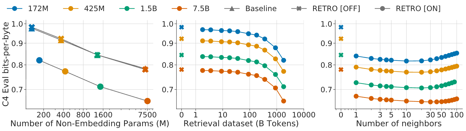
We show that our method scales well with model size and database size (Fig. 1): Retro provides a constant gain for models ranging from 150M to 7B parameters, and Retro can be improved at evaluation time by increasing the database size and the number of retrieved neighbours. Our largest model obtains state-of-the-art results on a range of downstream evaluation datasets including Wikitext103 (Merity et al., 2017) and the Pile (Gao et al., 2020) (§4). We show that Retro can be fine-tuned to achieve competitive performance on downstream tasks such as question answering (§4.3).
- •
We propose an evaluation aware of proximity of test documents with the training set (§2.6), addressing the problem of test set leakage (Lee et al., 2021). This is relevant for all language models, and especially for retrieval-enhanced models since they have direct access to the training dataset during evaluation. Using this methodology, we show that the performance of Retro comes from both explicit neighbour copying and general knowledge extraction (§4.4).
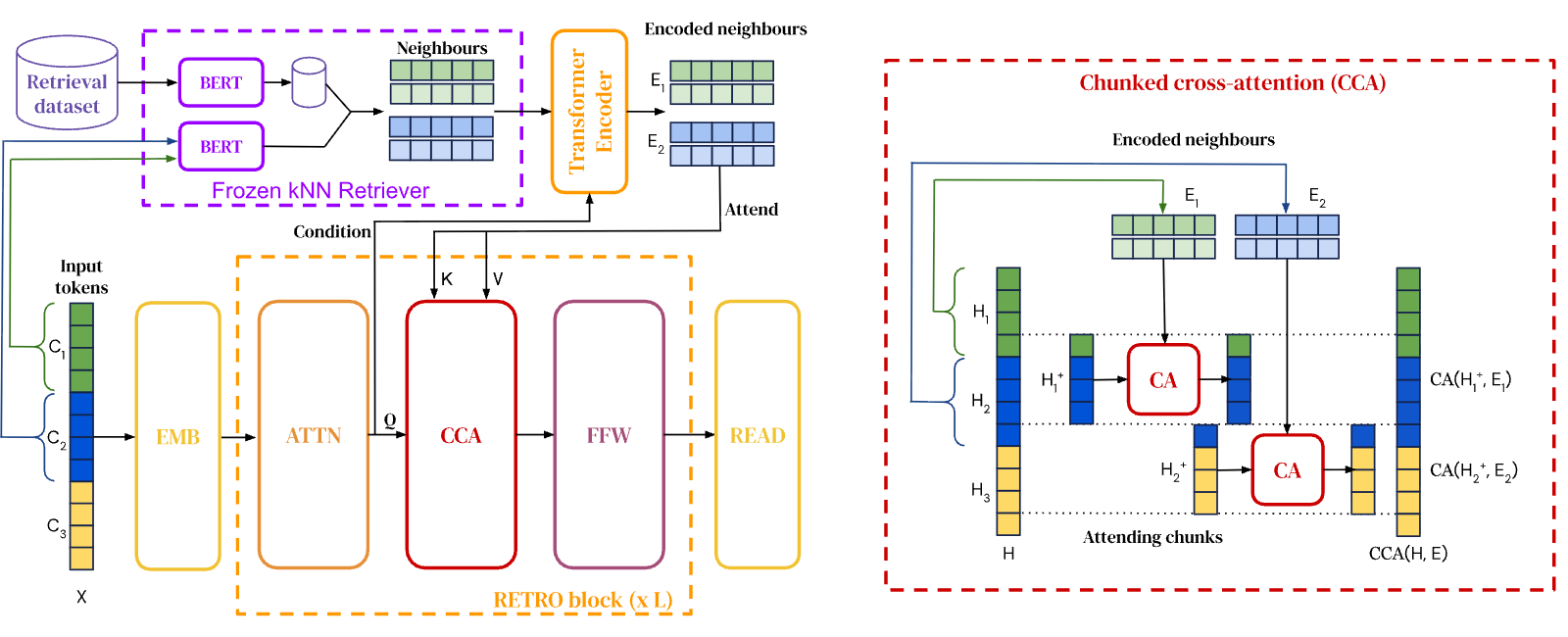
We design our retrieval-enhanced architecture to be capable of retrieving from a database with trillions of tokens. For this purpose, we retrieve at the level of contiguous token chunks instead of individual tokens which reduces storage and computation requirements by a large linear factor. Our method first constructs a key-value database, where values store raw chunks of text tokens and keys are frozen Bert embedddings (Devlin et al., 2019). We use a frozen model to avoid having to periodically re-compute embeddings over the entire database during training. Each training sequence is then split into chunks, which are augmented with their -nearest neighbour retrieved from the database. An encoder-decoder architecture integrates retrieval chunks into the model’s predictions. We summarize the Retro architecture in Fig. 2, and detail it in this section. We end the section by introducing a new methodology to evaluate language models when an evaluation set is partially present in the training set.
We use a multi-lingual version of MassiveText (Rae et al., 2021) for both training and retrieval data. The dataset consists of text documents from multiple sources and multiple languages totalling over 5 trillion tokens (detailed in Table 1). Sequences are sampled from subsets of the training data, with sampling weights given in the right-most column of Table 1. We tokenize the dataset using SentencePiece (Kudo and Richardson, 2018) with a vocabulary of 128,000 tokens. During training (unless otherwise specified), we retrieve from 600B tokens from the training data. The training retrieval database is made of the same subsets as the training data, in proportion that matches the training sampling frequencies. During evaluation the retrieval database consists in the full union of these datasets, with the exception of books for which we use a sub-sample of 4%. The evaluation retrieval database thus contains 1.75T tokens. To limit test set leakage, we compute the -gram Jaccard similarity between train and test documents using the MinHash scheme and remove all training documents with high similarity (0.8 or higher) to a validation or test set document. Additionally, we remove all validation and test articles from Wikitext103 (Merity et al., 2017) from our Wikipedia training data.
| Source | Token count (M) | Documents (M) | Multilingual | Sampling frequency |
|---|---|---|---|---|
| Web | 977,563 | 1,208 | Yes | 55% |
| Books | 3,423,740 | 20 | No | 25% |
| News | 236,918 | 398 | No | 10% |
| Wikipedia | 13,288 | 23 | Yes | 5% |
| GitHub | 374,952 | 143 | No | 5% |
View original table

Our approach uses retrieval as a way to augment input examples at the granularity of small chunks of tokens. Formally, we consider sequences of integer tokens in , obtained using a text tokenizer. We split each -token-long example into a sequence of chunks of size , i.e. . We use and . We augment each chunk with a set of neighbours from the database . (or Ret for brevity) is a non-trainable operator specified in §2.3. Token likelihoods are provided by a model, parameterized by , that takes as input both previous tokens and their retrieved neighbours. This defines the following retrieval-enhanced sequence log-likelihood:
We set , namely the likelihood of tokens from the first chunk does not depend on any retrieval data. This likelihood definition preserves autoregressivity: the probability of the -th token of the -th chunk, , only depends on previously seen tokens and on the data retrieved from the previous chunks . We can therefore directly sample with log-probability , where sampling within the chunk is conditioned on the neighbours . This makes retrieval-enhanced models directly comparable with the largest language models that are evaluated by sampling.
Our database consists of a key-value memory. Each value consists of two contiguous chunks of tokens which we denote where is the neighbour chunk which is used to compute the key, and is its continuation in the original document. The corresponding key is the Bert embedding of , averaged over time, that we denote . For each chunk , we retrieve its approximate -nearest neighbours from our key-value database using the distance on BERT embeddings . The model receives the corresponding values . Both neighbour chunks and their continuations provide meaningful improvements, as illustrated in our ablation study (Appendix D). We use a length for both and , thus has a shape of with . To avoid retrieving the chunk in the retrieval set , which would break causality during training, we filter out neighbours originating from the same document as the training sequence .
For a database of elements, we can query the approximate nearest neighbours in time. We use the SCaNN library (Guo et al., 2020) to achieve this. This means that we can query our trillion token database in whilst evaluating or sampling from the model; this expense is amortized over a chunk length. Performing retrieval on-the-fly is too slow to keep up with the training calculations—we leverage the frozen aspect of the embedding operator Bert to precompute all approximate nearest neighbours and save the results as part of the data. In Fig. 9 in the Appendix, we show results where we only retrieve neighbours within Wikipedia. We find that neighbours tend to come from 2-3 links away from a given article whereas random articles are more than 5 links apart.
Our model relies on an encoder-decoder transformer architecture, integrating the retrieved data through a cross-attention mechanism as introduced in Vaswani et al. (2017). First, the retrieved tokens are fed into an encoder Transformer, which computes the encoded neighbours set . Denoting the intermediate activations by , our transformer decoder then interleaves Retro-blocks and standard Transformer blocks (the hyperparameter determines at which layers we use a Retro-block). These blocks are built from three different residual operators with signature : a fully-connected layer Ffw, the standard sequence-level self-attention layer Attn, and a chunked cross-attention layer that incorporates information from the retrieval encoder:
Since Ffw, Attn and Cca are all autoregressive operators whose output at position only depends on , any succession of Retro and lm layers, followed by a token classification head defines an autoregressive log-likelihood (1). An overview of the model architecture is given in Algorithm 1 and in Fig. 2. We next describe the retrieval encoder and the chunked cross-attention layer in more detail, and explain how to sample from Retro.
For each chunk , the retrieval neighbours are fed into a bi-directional transformer Encoder, yielding the outputs , where indexes each neighbour. The retrieval encoder is a non-causal transformer. It is conditioned on , the activations of chunk , through cross-attention layers; this allows the representations of the retrieval encoder to be modulated by the retrieving chunk in a differentiable way. More precisely, the encoding of the j\textsuperscript{th} neighbour of the u\textsuperscript{th} chunk, , depends on the attended activation of chunk at layer . All neighbours for all chunks are encoded in parallel, yielding a full encoded set . We denote as the encoded neighbours for chunk .
To perform the Cca operation, we first split a given intermediate activation into attending chunks , as depicted on the right of Fig. 2. holds the intermediary embeddings of the last token in chunk and of the first tokens in . We compute the cross-attention between and —the encoded retrieval set obtained from chunk . Attention is computed across time and across neighbours simultaneously, as we merge the neighbour and time dimensions of before applying cross-attention. Since there is a notion of alignment between data chunks and retrieval neighbours, we use relative positional encodings as described in §B.1.2.
We concatenate the outputs of the per-chunk cross-attentions (each of shape ) across time, and properly pad the result; we thus form the output activation . Formally, for each chunk and for each token we set
where Ca is the cross-attention residual operator over time-concatenated encoded neighbours. We recall that this operator is defined in its simplest version by three parameter matrices and . For all and , we define
where the softmax is performed on the second dimension and all products are matrix products. We use multi-head cross-attention, and add positional encodings to the softmax(see §B.1.2).
The first tokens cannot attend to any neighbour of a previous chunk; at these positions, we define Cca as the identity, setting for all tokens . Finally, the last token attends to the last retrieval set and we set (not shown in Fig. 2). 1 contains a simplified implementation of Cca. Note that chunked cross-attention is autoregressive: the output of Cca at position depends on the sequence from tokens from to that is input to Cca.
With Retro models, even though each Cca cross-attention attends only to the neighbours of the preceding chunk , the dependencies over previous neighbours are propagated via the self-attention operations. The activations of the token in the chunk therefore potentially depend upon the set of all previous neighbours , without incurring the quadratic cost of cross attending to that set.
When sampling, at the end of a chunk , we use SCaNN to retrieve neighbours , based on the embedding . The encoded neighbours are then used to condition the generation of the next chunk , which we do incrementally: overall the cost of sampling is thus quadratic in the size of the sampled sequence, as when sampling from regular Transformers; the added cost of retrieval is linear in the number of chunks , and is negligible compared to the token sampling cost in practice.
We use a transformer (Vaswani et al., 2017) similar to the one described in (Radford et al., 2019), with some minimal changes: we replace LayerNorm with RMSNorm (Zhang and Sennrich, 2019) and use relative position encodings (Dai et al., 2019). As baselines, we train retrieval-free transformers with 132M, 368M, 1.3B and 7.0B parameters (embedding matrices are excluded from parameter counts). The hyperparameters we used are detailed in Table 2. All retrieval models use the same size encoder for the retrieval data, with and 2 layers, which roughly adds parameters. The encoder uses relative positional encodings. The retrieval models contain one Retro-block every 3 blocks, starting from layer 6. For our smallest model, Cca is applied in layers 6, 9 and 12 of the main pathway and also once for query conditioning in the encoder, which adds an additional parameters. The relative number of extra parameters reduces as we increase the baseline model size. All models are implemented using JAX (Bradbury et al., 2018) and Haiku (Hennigan et al., 2020).
| Baseline parameters | Retro | # heads | Head size | # layers | ||
|---|---|---|---|---|---|---|
| 132M | 172M (+30%) | 896 | 3,584 | 16 | 64 | 12 |
| 368M | 425M (+15%) | 1,536 | 6,144 | 12 | 128 | 12 |
| 1,309M | 1,451M (+11%) | 2,048 | 8,192 | 16 | 128 | 24 |
| 6,982M | 7,532M (+8%) | 4,096 | 16,384 | 32 | 128 | 32 |
View original table

Retro models may arguably benefit more easily from evaluation dataset leakage, i.e. the fact that we evaluate on data that were also present in the training set. To better understand how retrieval improves language modelling performance, we therefore quantify evaluation likelihood as a function of the overlap between the evaluation and training datasets.
The following approach can be used with any language model, and depends only on the frozen retriever system presented in §2.3. We split the evaluation sequences into chunks of length , and we see the training data as a set of chunks . For each evaluation chunk , we retrieve the 10 closest neighbours (of length up to 128) in the training data. We then compute the longest token substring common to both the evaluation chunk and its neighbours. This gives a number . The value , ranging from (chunk never seen) to (chunk entirely seen), gives a reliable indication of how much overlap there is between the evaluation chunk and the training data. For a given model, we then obtain the log-likelihood of each chunk , and the number of bytes it encodes. We then consider the filtered bits-per-bytes of the model:
which correspond to the bits-per-bytes on the set of chunks that overlap less than with the training chunks. Note that the full evaluation bit-per-bytes performance is recovered by . The function allows us to evaluate the impact of evaluation leakage over predictive performance: for low , gives an indication on how the model performs on chunks that are entirely new; the slope of shows how much the model exploits evaluation leakage.
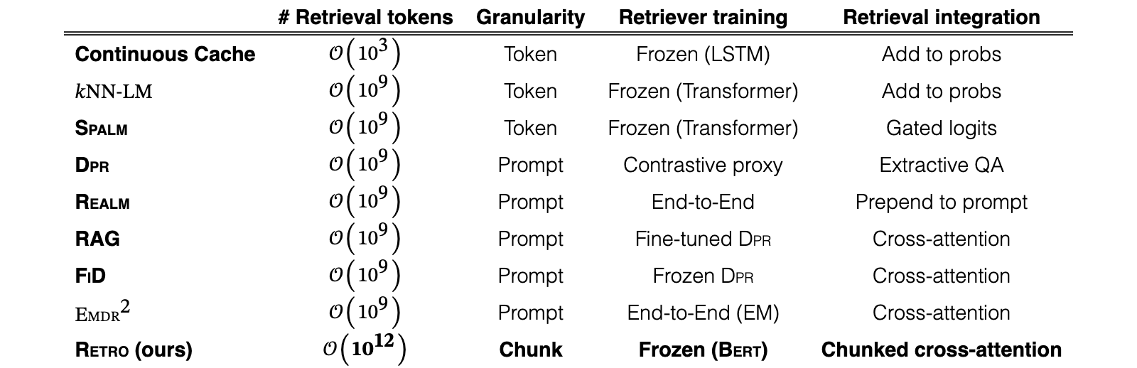
We first review existing work on using retrieval for language modelling, and compare Retro to these works (see Table 3). As we train Retro models on a large dataset containing a substantial section of the internet, our work raises potential privacy, safety, and fairness issues that we then review.
| # Retrieval tokens | Granularity | Retriever training | Retrieval integration | |
|---|---|---|---|---|
| Continuous Cache | Token | Frozen (LSTM) | Add to probs | |
| Token | Frozen (Transformer) | Add to probs | ||
| Spalm | Token | Frozen (Transformer) | Gated logits | |
| Dpr | Prompt | Contrastive proxy | Extractive QA | |
| Realm | Prompt | End-to-End | Prepend to prompt | |
| RAG | Prompt | Fine-tuned Dpr | Cross-attention | |
| FiD | Prompt | Frozen Dpr | Cross-attention | |
| Prompt | End-to-End (EM) | Cross-attention | ||
| Retro (ours) | Chunk | Frozen (Bert) | Chunked cross-attention |
View original table
Brants et al. (2007) show that scaling the training data to trillions of tokens improves the machine translation performance of -gram models. More recently, GPT-2 (Radford et al., 2019), GPT-3 (Brown et al., 2020), and Jurassic-1 (Lieber et al., 2021) show that scaling up language models leads to massive improvements on many downstream tasks. At the same time, Carlini et al. (2021) demonstrate that large-scale language models can perfectly memorise parts of their training data, suggesting that enhancing models with retrieval may lead to further improvements. However, significant leakage between train and test datasets (Lee et al., 2021; Lewis et al., 2021) makes comparing and evaluating large models trained on large datasets difficult, especially once retrieval capabilities over the training dataset are added.
Historically, information retrieval for text relies on inverted index matching such as TF-IDF and BM25 (Robertson and Zaragoza, 2009). Foundational work use latent topic modelling approaches like LDA (Blei et al., 2003) to identify relevant neighbours (Wei and Croft, 2006). Work in machine translation such as Zhang et al. (2018) and Gu et al. (2018) retrieve translation pairs based on edit distance between source sentences and guide the translation output using the closest retrieved target sentences. The retrieval database may also be structured — for example, Ahn et al. (2016) use a symbolic knowledge graph to improve an RNN language model.
With the success of deep learning, retrieving systems have partly switched to dense learned representations based on a neural network’s activations. Continuous cache (Grave et al., 2017) adds probability mass to tokens for which previous activations resemble the current activation vector, extending the model’s context to the local history. (Khandelwal et al., 2020) applies this idea to transformers and extends the retrieval database to English Wikipedia, resulting in substantial improvements on Wikitext103 evaluation. Continuous cache and do not modify the underlying neural-network models, but interpolate at inference between the language model’s output and distributions computed from retrieved tokens. These methods can therefore be plugged into any model without additional training, although this limits the model’s ability to reason about the retrieved text. Spalm (Yogatama et al., 2021) addresses this limitation by adding an extra gating network to post-process the retrieved data; yet most of the network is unaffected by the retrieval during inference.
The retrieval representations may be trained directly instead of relying on a pre-trained model—retriever systems have been developed for this purpose, primarily on open-domain question answering. For example, Dpr (Karpukhin et al., 2020) trains two Bert models (for queries and keys respectively) using a contrastive loss to align the representations of a question and of its answers. Lee et al. (2019) use an inverse cloze task to find semantic representations of passages for retrieval. These works differs from continuous cache and in that they embeds passages (or chunks) of text together, as opposed to each token individually. The retriever network is trained in isolation of the downstream task that uses the retrieval data. This potential issue is specifically addressed by Realm (Guu et al., 2020), which trains the retrieval system end-to-end to maximize the final training cross-entropy. This comes with the extra complexity of searching the database during training and periodically updating the embedding table, severely limiting the scale at which it can operate. RAG (Lewis et al., 2020) and FiD (Izacard and Grave, 2021) build upon Dpr to set the state of the art on question answering benchmarks by training encoder-decoder transformer models. More recently, (Sachan et al., 2021) extends FiD by using an expectation-maximization algorithm to train the retriever end-to-end and achieves state of the art results compared to similarly sized models.
In the open-domain dialogue setting, BlenderBot 2.0 (Komeili et al., 2021) learns to issue textual internet queries, outperforming dense retrieval methods when evaluated on a task measuring how close model responses are to those of humans. This involves collecting a dataset of human dialogues with associated search queries, which limits the scalability of this approach. Hashemi et al. (2020) introduce the Guided Transformer, a modified Transformer similar to Retro, for document retrieval and clarifying question selection. Although effective on question answering and other tasks with strong conditioning, none of these methods are designed to model arbitrary text sequences, in contrast with Retro.
Retro shares components with and Dpr in that it uses frozen retrieval representations. Retro models longer sequences than QA examples; this requires to reason at a sub-sequence level, and to retrieve different documents for the different chunks of a sequence. Similar to FiD, Retro processes the retrieved neighbours separately in the encoder, and assemble them in the chunked cross-attention. This differs from e.g. Realm, that prepends retrieved documents to the prompt. Using chunks allows for repeated retrieval whilst generating a sequence as opposed to retrieving only once based on the prompt alone. Furthermore, retrieval is done during the whole pre-training process in Retro, and is not simply plugged-in to solve a certain downstream task. Finally, previous methods based on dense query vectors use small models and retrieval datasets with less than 3B tokens (English Wikipedia). Table 3 summarizes the difference of Retro with existing approaches.
Bender et al. (2021); Weidinger et al. (2021) highlight several dangers of large language models. Those stem from their ability to memorise training data, their high training cost, the static nature of their training data (Lazaridou et al., 2021), their tendency of amplifying inherent biases in the training data, and their ability to generate toxic language (Gehman et al., 2020). In this section we inspect these dangers, focusing on how retrieval augmented language models may exacerbate or mitigate them.
Large language models can perfectly memorise parts of their training data (Carlini et al., 2021). When coupled with large training datasets gathered from the web or other sources, this has clear privacy and safety implications. Retrieval models such as Retro that have access to the entire training dataset during inference exacerbate these privacy issues by being able to directly copy training data. However, retrieval systems offer a path towards mitigating these concerns via obliteration of the retrievable data at inference time. In addition, differential privacy training (Abadi et al., 2016) of retrieval models could guarantee that no private information is stored in the model weights, while individualisation on private data could be made by updating the retrieval database at inference time.
Due to their high training cost, re-training large language model regularly to incorporate new data, languages, and norms is prohibitively expensive. To keep retrieval models up-to-date, it may be sufficient to update the retrieval database, which is orders of magnitude cheaper than re-training a model from scratch. In addition to the benefits of updating models in terms of fairness and bias, simply training large language models has a significant energy cost (Strubell et al., 2019; Schwartz et al., 2020). Retrieval mechanisms offer a path to reducing the compute requirements needed to train and update language models that reach a certain performance.
Large language models are prone to generating toxic outputs, as shown in Gehman et al. (2020). Bender et al. (2021); Jo and Gebru (2020) advocate for the importance of better training data curation and documentation. Additionally, if portions of the training data are found to be eliciting biased or toxic outputs after training, retrieval allows for some correction, as the offending retrieval data can be retroactively filtered. However, it is also the case that without careful analysis and intervention, retrieval models may exacerbate biases that are present in the training data. Retrieval models can also add a further source of bias through the selection mechanism for retrieval documents. Further work in this area is required to better understand how retrieval affects the bias and toxicity of the model outputs.
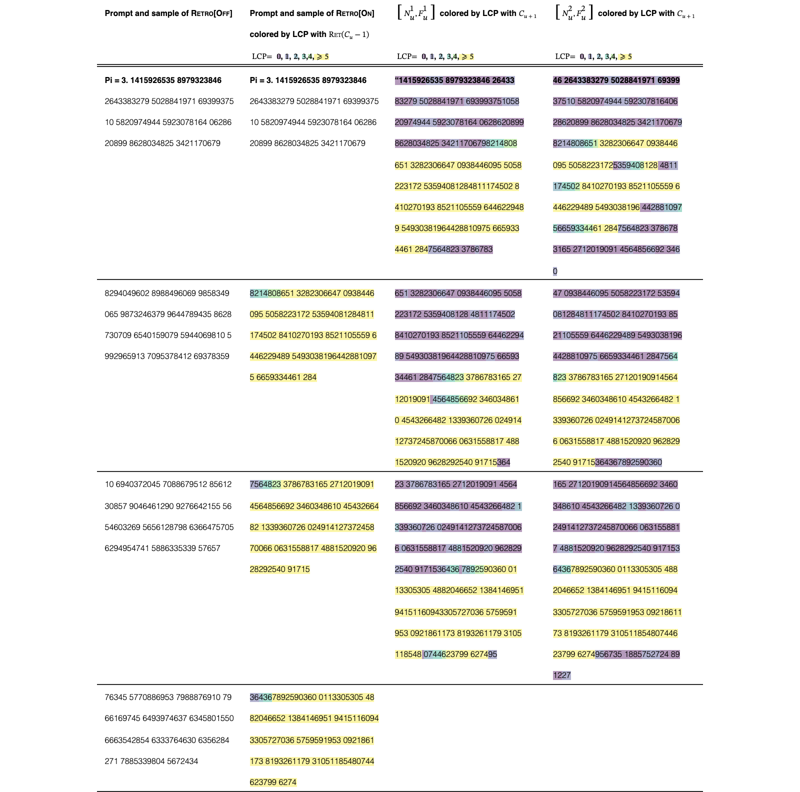
Finally, samples from large models are difficult to interpret, making mitigating these issues all the more challenging (Belinkov et al., 2020; Jain and Wallace, 2019). Retrieval provides more insights in to the outputs of a model, as one can directly visualise or modify the neighbours that are being used. The examples in Table 6, 7, 20 and 21 illustrate how retrieval makes language models more factual and interpretable by providing more transparent outputs.
We first report results on language modelling benchmarks. Second, we show how to Retrofit pre-trained Transformer language models into retrieval models with few additional FLOPs. Next, we report Retro results on question answering. Finally, we report evaluation metrics with leakage filtering, to better understand the source of the gains with retrieval.
We evaluate our models on C4 (Raffel et al., 2020), Wikitext103 (Merity et al., 2017), Curation Corpus (Curation, 2020), Lambada (Paperno et al., 2016) and the Pile (Gao et al., 2020). We also evaluate on a set of manually selected Wikipedia articles that were added or heavily edited in September 2021, months after our pre-training and retrieval dataset was collected (details are given in §A.2). We construct the dataset with articles from the “future” and manually remove new articles that strongly overlap documents in our training data. This guarantees that the evaluation documents are not leaked in our training data.
For C4, Wikitext103, the Pile, and our Wikipedia dataset we evaluate the language modelling performance on entire documents and measure the bits-per-byte (bpb). We favour bits-per-byte over loss as it is tokenizer agnostic. We evaluate with a sequence length of 2048 tokens but use a stride of 1024 within documents to mitigate boundary effects. On Curation Corpus we concatenate the article, the “TL;DR:” string, and the summary, but only evaluate the bpb on the summary. For Lambada we evaluate the accuracy on the last word, using greedy generation.
In Fig. 1(left) and Fig. 3 we show the language modelling performance as we scale models from 150 million to 7 billion (non-embedding) parameters. We see that on all datasets, Retro outperforms the baseline at all model sizes. Furthermore, we observe that improvements do not diminish as we scale the models. The performance is dataset dependent, with the largest gains on Wikitext103 and C4. Wikipedia articles and other web pages are similar to Wikitext103 documents, even if not exact copies (§4.4), we thus obtain dramatic improvements on Wikitext103 as our retrieval model is able to directly exploit these overlaps. The smallest gains are for Curation Corpus, where Retro only slightly outperforms the baseline. This is expected as Curation Corpus summaries are designed to only contain information from the source article and are not included in our retrieval database. On our “future” Wikipedia September 2021 dataset, we also observe consistent gains for all model sizes.
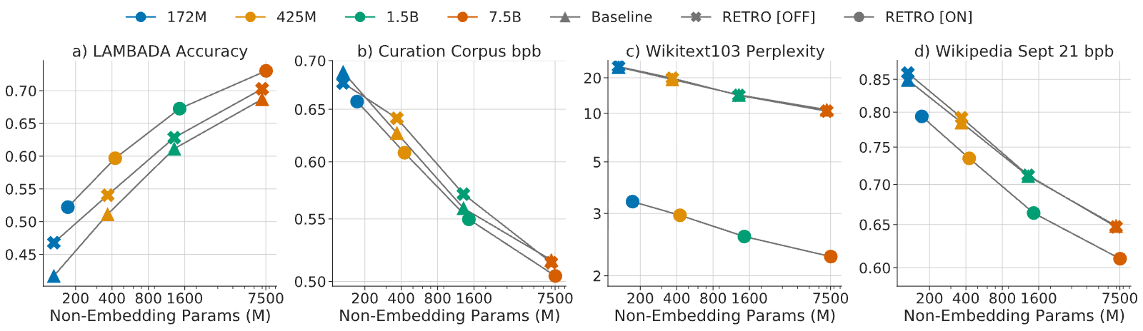
Fig. 1 (middle) shows how scaling the retrieval database at evaluation improves the language modelling performance. We observe dramatic gains as the retrieval data is increased from Wikipedia (4 billion tokens) to all of Massive text (1.7T tokens). Fig. 1(right) shows how performance scales as we increase the number of retrieved chunks. Despite being only trained with 2 neighbours, we see consistent improvements for all models when the number of neighbours is increased from 1 to 10. Furthermore, we observe that larger models are able to better utilise more neighbours: the 172M model improves with up to 10 neighbours, whereas the 7B model improves with up to 40 neighbours.
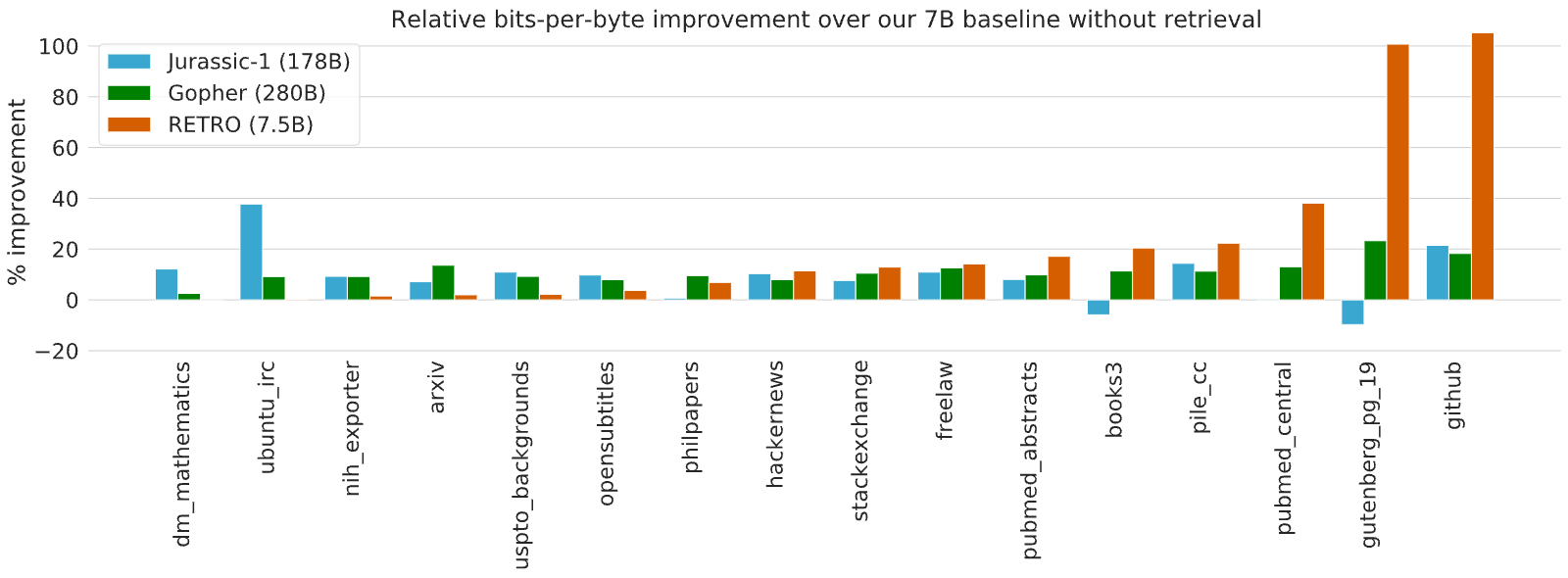
We evaluate our 7B models on the Pile test sets and compare against the 178B parameter Jurrasic-1 (Lieber et al., 2021) model and the 280B parameter Gopher (Rae et al., 2021) model. We do not compare against GPT-3 as it is outperformed by Jurassic-1 and Gopher on almost all subsets. Fig. 4 shows the relative improvements in bits-per-byte over our 7B transformer baseline for our 7.5B Retro model, Jurassic-1 and Gopher. Jurassic-1 outperforms the baseline on all datasets except for books, likely due to the inclusion of books in our training data. Gopher and Retro outperform the baseline on all test sets. Overall, Retro 7.5B outperforms Jurassic-1 and Gopher on a majority of the test sets. On the dm_mathematics and ubuntu_irc subsets, our Retro model does not outperform our 7B baseline and underperforms Jurassic-1. We hypothesise that the retrieved neighbours on these datasets are not helpful, due to a combination of what is in our retrieval dataset and the efficacy of the nearest-neighbour search.
| Model | Retrieval Set | #Database tokens | #Database keys | Valid | Test |
|---|---|---|---|---|---|
| Adaptive Inputs (Baevski and Auli, 2019) | - | - | - | 17.96 | 18.65 |
| Spalm (Yogatama et al., 2021) | Wikipedia | 3B | 3B | 17.20 | 17.60 |
| (Khandelwal et al., 2020) | Wikipedia | 3B | 3B | 16.06 | 16.12 |
| Megatron (Shoeybi et al., 2019) | - | - | - | - | 10.81 |
| Baseline transformer (ours) | - | - | - | 21.53 | 22.96 |
| (ours) | Wikipedia | 4B | 4B | 18.52 | 19.54 |
| Retro | Wikipedia | 4B | 0.06B | 18.46 | 18.97 |
| Retro | C4 | 174B | 2.9B | 12.87 | 10.23 |
| Retro | MassiveText (1%) | 18B | 0.8B | 18.92 | 20.33 |
| Retro | MassiveText (10%) | 179B | 4B | 13.54 | 14.95 |
| Retro | MassiveText (100%) | 1792B | 28B | 3.21 | 3.92 |
View original table
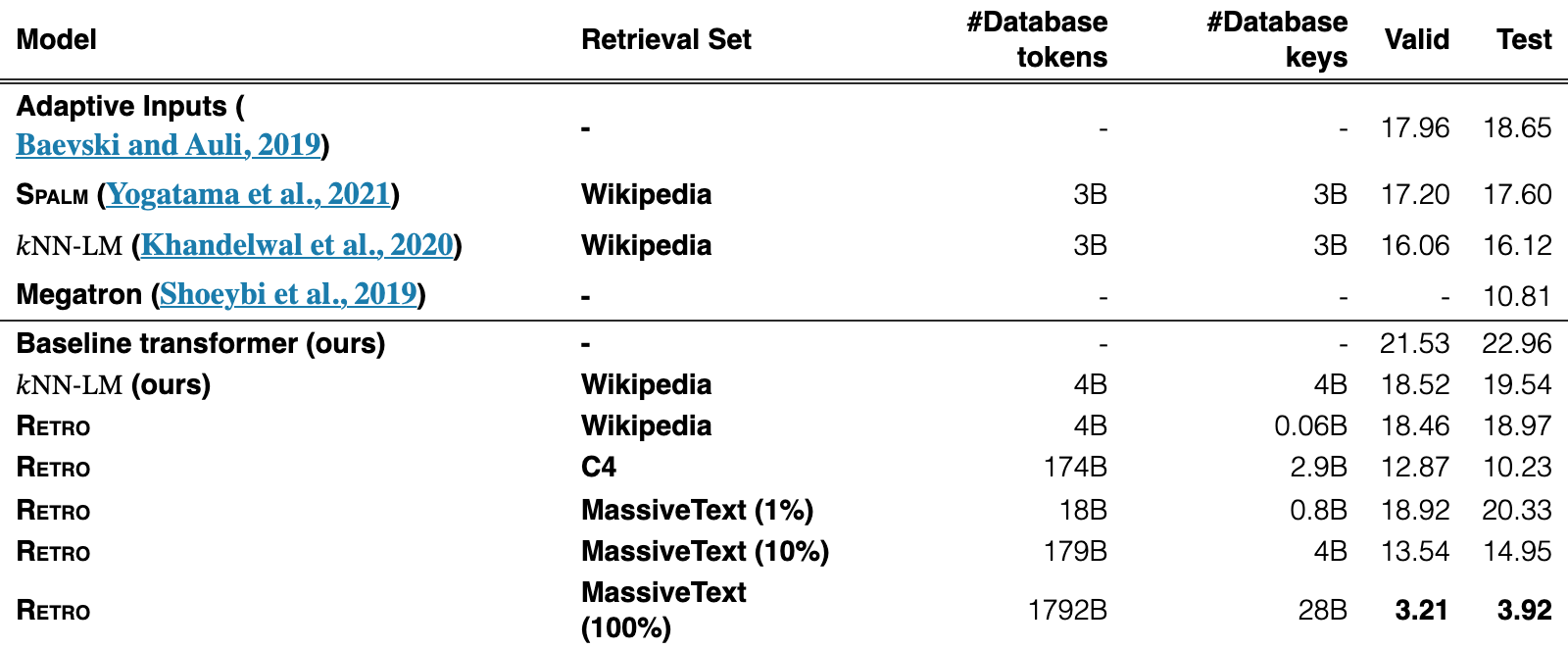
To validate our approach in a controlled setting, we compare our method with (Khandelwal et al., 2020) on the Wikitext103 dataset in Table 4. We train a baseline transformer on the training set of Wikitext103. This transformer has 24 layers, 1024 hidden units, 16 heads and a key size of 64, as in Baevski and Auli (2019). Our baseline does not have adaptive input, and our tokenizer has an open vocabulary, unlike Baevski and Auli (2019), which makes our baseline perplexities a bit higher. The full experiment details and hyperparameters are given in §C.2 and Table 11.
We re-implement with our tokenizer and baseline transformer to produce embeddings of size 1024 for every token in Wikitext103. has probabilities with . We tune and on the validation set (Fig. 7) and report performance for these hyperparameters on both the validation and test set.
We fine-tune our baseline transformer into a Retro model (Fig. 7), using the Wikitext103 training data and retrieving from Wikipedia with 2 neighbours. We only train the new weights, as explained in §4.2, and share the embedding weights between the encoder and the main pathway. This is necessary for Wikitext103 which is quite small, as training Retro from scratch in this setting leads to over-fitting.
We evaluate the fine-tuned Retro model with different retrieval sets. We use 10 neighbours at evaluation for both Retro and . When retrieving from Wikipedia, we obtain results comparable to our implementation. Furthermore, scaling the retrieval database to MassiveText yields dramatic improvements, though this is partly due to leakage (see §4.4). For reproducibility, we also include results when retrieving from C4, which are close to previous state-of-the-art and comparable to using 10 % of MassiveText.
It is worth noting that requires 1024 floats for every token in the retrieval dataset, totalling 15 terabytes (Tb) for the 4 billion tokens in Wikipedia. and other token-level retrieval approaches therefore don’t scale to retrieval databases with trillions of tokens such as MassiveText. In comparison, Retro only requires 215Gb to index our Wikipedia dataset, and 93Tb for MassiveText. Inspecting the number of retrieval database entries in Table 4 makes it clear why retrieving at the chunk level is necessary when scaling to datasets with trillions of tokens.
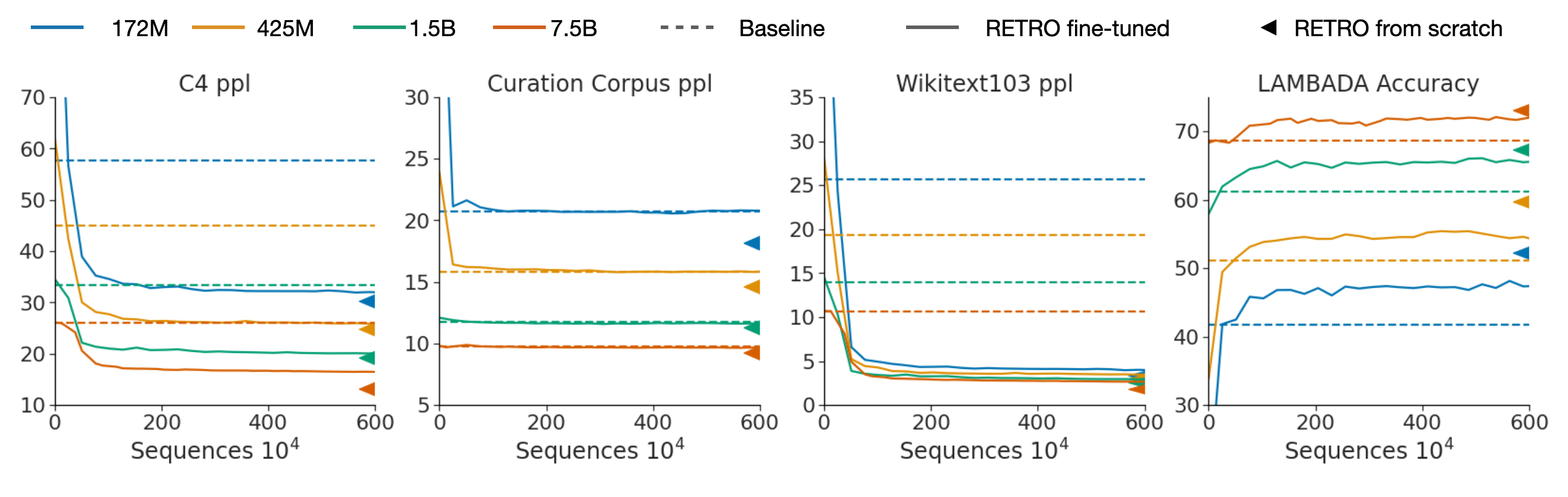
We extend baseline models into Retro models by freezing the pre-trained weights and training only chunked cross-attention and neighbour encoder parameters (less than 10% of weights for the 7B model) in Fig. 5. This offers an efficient alternative path to enhance transformers with retrieval, requiring only 6 million sequences (3% of the pre-training sequences that we used). Additionally, by only training the new weights we ensure that when evaluated without retrieval, the original model performance is exactly maintained. Retrofitting models quickly surpasses the performance of baseline models and even achieves performance close to that of Retro models trained from scratch. The experiment hyperparameters are given in §C.3.
We fine-tune our retrieval models on the Natural Questions (Kwiatkowski et al., 2019) dataset to demonstrate that our retrieval pathway can be used to inject information from arbitrary data sources. We use the version provided by Izacard and Grave (2021) which is augmented with the retrieved passages from Dpr (Karpukhin et al., 2020). We fine-tune all the weights of our 7.5B pre-trained Retro model for 25,000 steps using the top 20 retrieved passages. We format the data as “question: {question} \n answer: {answer}” and left pad the data such that “answer:” coincides with the end of the first chunk of 64 tokens and thus aligns with the first retrieving chunk. The model has access to the question via the previous tokens in the sequence as well as the top 20 DPR Wikipedia passages and their titles via the chunked cross-attention mechanism. The exact match scores are shown in Table 5 and the full fine-tuning details are given in §C.4. Our method is competitive with previous approaches such as Realm, RAG and Dpr, but underperforms the more recent FiD. In contrast with this work, we find that increasing the number of neighbours past 20 does not improve Retro performance on this task. We hypothesise that the encoder-decoder structure of T5—the base model in FiD— and the T5 pre-training objective leads to a model that relies more on the encoder output than Retro, which is important in the QA setting. To compete with T5-finetuned models, future work should consider ways of forcing Retro to rely further on the retrieval encoder output when producing tokens.
| Model | Test Accuracy |
|---|---|
| Realm (Guu et al., 2020) | 40.4 |
| Dpr (Karpukhin et al., 2020) | 41.5 |
| RAG (Lewis et al., 2020) | 44.5 |
| (Sachan et al., 2021) | 52.5 |
| FiD (Izacard and Grave, 2021) | 51.4 |
| FiD + Distill. (Izacard et al., 2020) | 54.7 |
| Baseline 7B (closed book) | 30.4 |
| Retro 7.5B (DPR retrieval) | 45.5 |
View original table

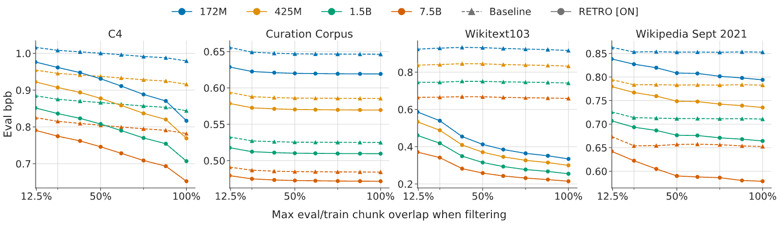
We report the filtered eval losses as detailed in §2.6 on C4, Curation Corpus and Wikitext103 in Fig. 6. On C4 and Wikitext103, for which there is leakage into the training set, the slope is negative for both baseline models and Retro models. Retro models exploit leakage more strongly than baseline models, as indicated by the more negative slope. This is due to its explicit ability to copy-paste existing training chunks to predict leaked evaluation chunks (see a qualitative example of this model behavior on a Wikitext103 article in Table 19). On Curation Corpus, retrieval provides a constant offset, which is expected as there is by design no leakage between Curation Corpus and the training dataset.
On the other hand, Retro outperforms baseline models at all leakage levels, down to . At this level, the loss is computed on chunks with less than contiguous tokens shared with the closest matching chunk in the training dataset—this is a reasonable level of overlap at which we consider that there is no local leakage. Retrieval thus improves predictions on both chunks that are syntactically similar to chunks in the training set, and on chunks that are syntactically different from all training chunks. This points toward a non trivial Retro capacity of generalizing based on both model parameters and retrieval database. Similar results are found on the Pile dataset (see Fig. 12, §F.3).
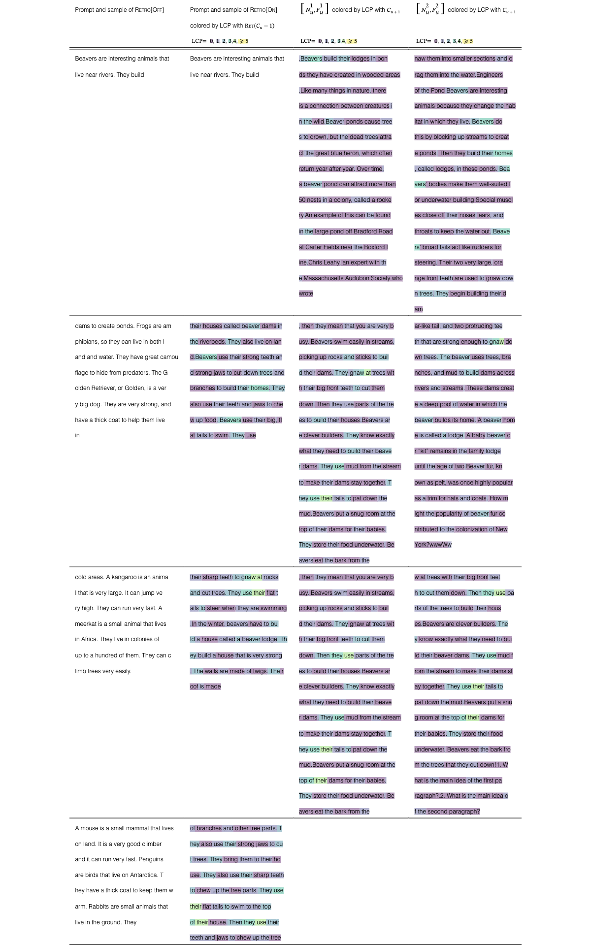
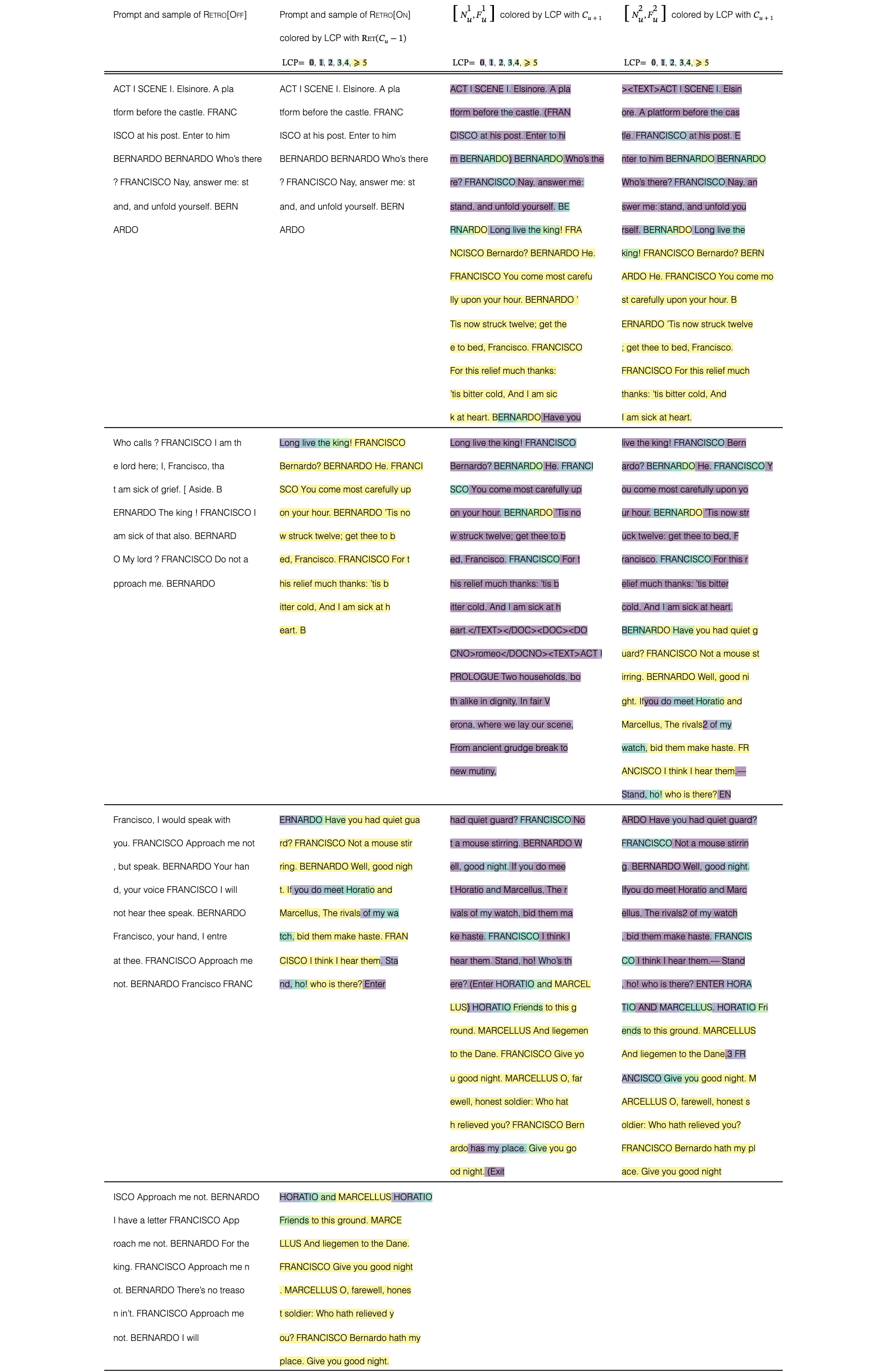
We show examples of samples obtained using the 7.5B Retro model in Table 6, Table 7 and Appendix E. For each chunk (the first one being the prompt), we juxtapose sampled chunks with retrieved neighbours . To give an indication of local overlap, we colour each sampled token in chunk based on the length of the longest common prefix (LCP) found in the retrieved chunks . Similarly, we colour the retrieved chunks based on the LCP in the sampled chunk. For the sample in Table 6, for which we chose the prompt, we observe that the retrieved chunks influence the sample as there are overlaps between the sampled tokens and neighbour tokens. Overall, retrieval reduces hallucinations (in line with the findings of Shuster et al. (2021)) and makes the model more knowledgeable, when comparing with samples produced with retrieval disabled. In the sample in Table 7, the model recognises that the prompt is the beginning of the first scene of Hamlet and leverages retrieval data to continue it with only a few mistakes. We provide further examples in Appendix E, including examples from the evaluation sets, as well as the detailed procedure used for colouring the tables.
We present Retrieval-Enhanced Transformers (Retro), a method for modelling arbitrary text sequences whilst retrieving from databases with trillions of tokens—scaling the data available to models by an order of magnitude compared to what is typically consumed during training. Retro models gains do not diminish for models with up to at least 7B parameters, and correspond to non-retrieval models with 10 more parameters on certain datasets. On Wikitext103 and the Pile, Retro outperforms previous models trained on large scale datasets. We also show that Retro is competitive on retrieval-intensive downstream tasks such as question answering.
Retro models are flexible and can be used without retrieval at evaluation and still achieve comparable performance to baseline models. Conversely, baseline models can be rapidly fine-tuned into Retro models to obtain nearly the same performance as if trained from scratch. Careful analysis shows that only a modest fraction of the gains obtained by Retro are due to test set leakage. In general, we caution for such leakage in large-scale language datasets and suggest further work in better understanding the role of test set leakage in the performance of large-scale language models.
Overall, our work demonstrates at an unprecedented scale that semi-parametric approaches can provide an orthogonal, more efficient approach than raw parameter scaling as we seek to build more powerful language models.
We would like to thank Nikolai Grigorev, Marc’aurelio Ranzato, Cyprien de Masson d’Autume, Po-Sen Huang, Johannes Welbl, Lisa Anne Hendricks, Ethan Perez, Jeff Stanway, Eric Noland, Gregory Wayne, John Jumper, Julian Schrittwieser, Lorrayne Bennett, Devang Agrawal, Dani Yogatama, Susannah Young, Nando de Freitas, Demis Hassabis, and Koray Kavukcuoglu for their help, advice and reviews. Additionally, we would like to thank Zonglin Li, David Simcha, and the ScaNN developers for their help.
| Prompt and sample of Retro[Off] | Prompt and sample of Retro[On] | colored by LCP with | colored by LCP with |
| colored by LCP with | |||
| , , , ,, | , , , ,, | , , , ,, | |
| Beavers are interesting animals that | Beavers are interesting animals that | .Beavers build their lodges in pon | naw them into smaller sections and d |
| live near rivers. They build | live near rivers. They build | ds they have created in wooded areas | rag them into the water.Engineers |
| .Like many things in nature, there | of the Pond Beavers are interesting | ||
| is a connection between creatures i | animals because they change the hab | ||
| n the wild.Beaver ponds cause tree | itat in which they live. Beavers do | ||
| s to drown, but the dead trees attra | this by blocking up streams to creat | ||
| ct the great blue heron, which often | e ponds. Then they build their homes | ||
| return year after year. Over time, | , called lodges, in these ponds. Bea | ||
| a beaver pond can attract more than | vers’ bodies make them well-suited f | ||
| 50 nests in a colony, called a rooke | or underwater building Special muscl | ||
| ry.An example of this can be found | es close off their noses, ears, and | ||
| in the large pond off Bradford Road | throats to keep the water out. Beave | ||
| at Carter Fields near the Boxford l | rs’ broad tails act like rudders for | ||
| ine.Chris Leahy, an expert with th | steering. Their two very large, ora | ||
| e Massachusetts Audubon Society who | nge front teeth are used to gnaw dow | ||
| wrote | n trees. They begin building their d | ||
| am | |||
| dams to create ponds. Frogs are am | their houses called beaver dams in | , then they mean that you are very b | ar-like tail, and two protruding tee |
| phibians, so they can live in both l | the riverbeds. They also live on lan | usy. Beavers swim easily in streams, | th that are strong enough to gnaw do |
| and and water. They have great camou | d.Beavers use their strong teeth an | picking up rocks and sticks to buil | wn trees. The beaver uses trees, bra |
| flage to hide from predators. The G | d strong jaws to cut down trees and | d their dams. They gnaw at trees wit | nches, and mud to build dams across |
| olden Retriever, or Golden, is a ver | branches to build their homes. They | h their big front teeth to cut them | rivers and streams. These dams creat |
| y big dog. They are very strong, and | also use their teeth and jaws to che | down. Then they use parts of the tre | e a deep pool of water in which the |
| have a thick coat to help them live | w up food. Beavers use their big, fl | es to build their houses.Beavers ar | beaver builds its home. A beaver hom |
| in | at tails to swim. They use | e clever builders. They know exactly | e is called a lodge. A baby beaver o |
| what they need to build their beave | r “kit” remains in the family lodge | ||
| r dams. They use mud from the stream | until the age of two.Beaver fur, kn | ||
| to make their dams stay together. T | own as pelt, was once highly popular | ||
| hey use their tails to pat down the | as a trim for hats and coats. How m | ||
| mud.Beavers put a snug room at the | ight the popularity of beaver fur co | ||
| top of their dams for their babies. | ntributed to the colonization of New | ||
| They store their food underwater. Be | York?wwwWw | ||
| avers eat the bark from the | |||
| cold areas. A kangaroo is an anima | their sharp teeth to gnaw at rocks | , then they mean that you are very b | w at trees with their big front teet |
| l that is very large. It can jump ve | and cut trees. They use their flat t | usy. Beavers swim easily in streams, | h to cut them down. Then they use pa |
| ry high. They can run very fast. A | ails to steer when they are swimming | picking up rocks and sticks to buil | rts of the trees to build their hous |
| meerkat is a small animal that lives | .In the winter, beavers have to bui | d their dams. They gnaw at trees wit | es.Beavers are clever builders. The |
| in Africa. They live in colonies of | ld a house called a beaver lodge. Th | h their big front teeth to cut them | y know exactly what they need to bui |
| up to a hundred of them. They can c | ey build a house that is very strong | down. Then they use parts of the tre | ld their beaver dams. They use mud f |
| limb trees very easily. | . The walls are made of twigs. The r | es to build their houses.Beavers ar | rom the stream to make their dams st |
| oof is made | e clever builders. They know exactly | ay together. They use their tails to | |
| what they need to build their beave | pat down the mud.Beavers put a snu | ||
| r dams. They use mud from the stream | g room at the top of their dams for | ||
| to make their dams stay together. T | their babies. They store their food | ||
| hey use their tails to pat down the | underwater. Beavers eat the bark fro | ||
| mud.Beavers put a snug room at the | m the trees that they cut down!1. W | ||
| top of their dams for their babies. | hat is the main idea of the first pa | ||
| They store their food underwater. Be | ragraph?.2. What is the main idea o | ||
| avers eat the bark from the | f the second paragraph? | ||
| A mouse is a small mammal that lives | of branches and other tree parts. T | ||
| on land. It is a very good climber | hey also use their strong jaws to cu | ||
| and it can run very fast. Penguins | t trees. They bring them to their ho | ||
| are birds that live on Antarctica. T | use. They also use their sharp teeth | ||
| hey have a thick coat to keep them w | to chew up the tree parts. They use | ||
| arm. Rabbits are small animals that | their flat tails to swim to the top | ||
| live in the ground. They | of their house. Then they use their | ||
| teeth and jaws to chew up the tree |
View original table
| Prompt and sample of Retro[Off] | Prompt and sample of Retro[On] | colored by LCP with | colored by LCP with |
| colored by LCP with | |||
| , , , ,, | , , , ,, | , , , ,, | |
| ACT I SCENE I. Elsinore. A pla | ACT I SCENE I. Elsinore. A pla | ACT I SCENE I. Elsinore. A pla | ><TEXT>ACT I SCENE I. Elsin |
| tform before the castle. FRANC | tform before the castle. FRANC | tform before the castle. (FRAN | ore. A platform before the cas |
| ISCO at his post. Enter to him | ISCO at his post. Enter to him | CISCO at his post. Enter to hi | tle. FRANCISCO at his post. E |
| BERNARDO BERNARDO Who’s there | BERNARDO BERNARDO Who’s there | m BERNARDO) BERNARDO Who’s the | nter to him BERNARDO BERNARDO |
| ? FRANCISCO Nay, answer me: st | ? FRANCISCO Nay, answer me: st | re? FRANCISCO Nay, answer me: | Who’s there? FRANCISCO Nay, an |
| and, and unfold yourself. BERN | and, and unfold yourself. BERN | stand, and unfold yourself. BE | swer me: stand, and unfold you |
| ARDO | ARDO | RNARDO Long live the king! FRA | rself. BERNARDO Long live the |
| NCISCO Bernardo? BERNARDO He. | king! FRANCISCO Bernardo? BERN | ||
| FRANCISCO You come most carefu | ARDO He. FRANCISCO You come mo | ||
| lly upon your hour. BERNARDO ’ | st carefully upon your hour. B | ||
| Tis now struck twelve; get the | ERNARDO ’Tis now struck twelve | ||
| e to bed, Francisco. FRANCISCO | ; get thee to bed, Francisco. | ||
| For this relief much thanks: | FRANCISCO For this relief much | ||
| ’tis bitter cold, And I am sic | thanks: ’tis bitter cold, And | ||
| k at heart. BERNARDO Have you | I am sick at heart. | ||
| Who calls ? FRANCISCO I am th | Long live the king! FRANCISCO | Long live the king! FRANCISCO | live the king! FRANCISCO Bern |
| e lord here; I, Francisco, tha | Bernardo? BERNARDO He. FRANCI | Bernardo? BERNARDO He. FRANCI | ardo? BERNARDO He. FRANCISCO Y |
| t am sick of grief. [ Aside. B | SCO You come most carefully up | SCO You come most carefully up | ou come most carefully upon yo |
| ERNARDO The king ! FRANCISCO I | on your hour. BERNARDO ’Tis no | on your hour. BERNARDO ’Tis no | ur hour. BERNARDO ’Tis now str |
| am sick of that also. BERNARD | w struck twelve; get thee to b | w struck twelve; get thee to b | uck twelve: get thee to bed, F |
| O My lord ? FRANCISCO Do not a | ed, Francisco. FRANCISCO For t | ed, Francisco. FRANCISCO For t | rancisco. FRANCISCO For this r |
| pproach me. BERNARDO | his relief much thanks: ’tis b | his relief much thanks: ’tis b | elief much thanks: ’tis bitter |
| itter cold, And I am sick at h | itter cold, And I am sick at h | cold, And I am sick at heart. | |
| eart. B | eart.</TEXT></DOC><DOC><DO | BERNARDO Have you had quiet g | |
| CNO>romeo</DOCNO><TEXT>ACT I | uard? FRANCISCO Not a mouse st | ||
| PROLOGUE Two households, bo | irring. BERNARDO Well, good ni | ||
| th alike in dignity, In fair V | ght. Ifyou do meet Horatio and | ||
| erona, where we lay our scene, | Marcellus, The rivals2 of my | ||
| From ancient grudge break to | watch, bid them make haste. FR | ||
| new mutiny, | ANCISCO I think I hear them.— | ||
| Stand, ho! who is there? EN | |||
| Francisco, I would speak with | ERNARDO Have you had quiet gua | had quiet guard? FRANCISCO No | ARDO Have you had quiet guard? |
| you. FRANCISCO Approach me not | rd? FRANCISCO Not a mouse stir | t a mouse stirring. BERNARDO W | FRANCISCO Not a mouse stirrin |
| , but speak. BERNARDO Your han | ring. BERNARDO Well, good nigh | ell, good night. If you do mee | g. BERNARDO Well, good night. |
| d, your voice FRANCISCO I will | t. If you do meet Horatio and | t Horatio and Marcellus, The r | Ifyou do meet Horatio and Marc |
| not hear thee speak. BERNARDO | Marcellus, The rivals of my wa | ivals of my watch, bid them ma | ellus, The rivals2 of my watch |
| Francisco, your hand, I entre | tch, bid them make haste. FRAN | ke haste. FRANCISCO I think I | , bid them make haste. FRANCIS |
| at thee. FRANCISCO Approach me | CISCO I think I hear them. Sta | hear them. Stand, ho! Who’s th | CO I think I hear them.— Stand |
| not. BERNARDO Francisco FRANC | nd, ho! who is there? Enter | ere? (Enter HORATIO and MARCEL | , ho! who is there? ENTER HORA |
| LUS) HORATIO Friends to this g | TIO AND MARCELLUS. HORATIO Fri | ||
| round. MARCELLUS And liegemen | ends to this ground. MARCELLUS | ||
| to the Dane. FRANCISCO Give yo | And liegemen to the Dane.3 FR | ||
| u good night. MARCELLUS O, far | ANCISCO Give you good night. M | ||
| ewell, honest soldier: Who hat | ARCELLUS O, farewell, honest s | ||
| h relieved you? FRANCISCO Bern | oldier: Who hath relieved you? | ||
| ardo has my place. Give you go | FRANCISCO Bernardo hath my pl | ||
| od night. (Exit | ace. Give you good night | ||
| ISCO Approach me not. BERNARDO | HORATIO and MARCELLUS HORATIO | ||
| I have a letter FRANCISCO App | Friends to this ground. MARCE | ||
| roach me not. BERNARDO For the | LLUS And liegemen to the Dane. | ||
| king. FRANCISCO Approach me n | FRANCISCO Give you good night | ||
| ot. BERNARDO There’s no treaso | . MARCELLUS O, farewell, hones | ||
| n in’t. FRANCISCO Approach me | t soldier: Who hath relieved y | ||
| not. BERNARDO I will | ou? FRANCISCO Bernardo hath my | ||
| place. Give you good night. |
View original table
References
- Abadi et al. (2016) M. Abadi, A. Chu, I. Goodfellow, H. B. McMahan, I. Mironov, K. Talwar, and L. Zhang. Deep learning with differential privacy. In ACM SIGSAC Conference on Computer and Communications Security, 2016.
- Ahn et al. (2016) S. Ahn, H. Choi, T. Pärnamaa, and Y. Bengio. A neural knowledge language model. arXiv preprint arXiv:1608.00318, 2016.
- Baevski and Auli (2019) A. Baevski and M. Auli. Adaptive input representations for neural language modeling. In International Conference on Learning Representations, 2019. URL https://openreview.net/forum?id=ByxZX20qFQ.Source
- Belinkov et al. (2020) Y. Belinkov, S. Gehrmann, and E. Pavlick. Interpretability and analysis in neural NLP. In Proceedings of the 58th Annual Meeting of the Association for Computational Linguistics: Tutorial Abstracts, pages 1–5, Online, July 2020. Association for Computational Linguistics. 10.18653/v1/2020.acl-tutorials.1. URL https://aclanthology.org/2020.acl-tutorials.1.SourceSource
- Bender et al. (2021) E. M. Bender, T. Gebru, A. McMillan-Major, and S. Shmitchell. On the dangers of stochastic parrots: Can language models be too big? In ACM Conference on Fairness, Accountability, and Transparency, 2021.
- Blei et al. (2003) D. M. Blei, A. Y. Ng, and M. I. Jordan. Latent Dirichlet Allocation. Journal of Machine Learning Research, 3(Jan):993–1022, 2003. URL https://jmlr.csail.mit.edu/papers/v3/blei03a.html.Source
- Bradbury et al. (2018) J. Bradbury, R. Frostig, P. Hawkins, M. J. Johnson, C. Leary, D. Maclaurin, G. Necula, A. Paszke, J. V. der Plas, S. Wanderman-Milne, and Q. Zhang. JAX: composable transformations of Python+NumPy programs, 2018. URL http://github.com/google/jax.Source
- Brants et al. (2007) T. Brants, A. C. Popat, P. Xu, F. J. Och, and J. Dean. Large Language models in machine translation. In Joint Conference on Empirical Methods in Natural Language Processing and Computational Natural Language Learning, pages 858–867, 2007.
- Brown et al. (2020) T. Brown, B. Mann, N. Ryder, M. Subbiah, J. D. Kaplan, P. Dhariwal, A. Neelakantan, P. Shyam, G. Sastry, A. Askell, S. Agarwal, A. Herbert-Voss, G. Krueger, T. Henighan, R. Child, A. Ramesh, D. Ziegler, J. Wu, C. Winter, C. Hesse, M. Chen, E. Sigler, M. Litwin, S. Gray, B. Chess, J. Clark, C. Berner, S. McCandlish, A. Radford, I. Sutskever, and D. Amodei. Language models are few-shot learners. In Advances in Neural Information Processing Systems, 2020. URL https://proceedings.neurips.cc/paper/2020/file/1457c0d6bfcb4967418bfb8ac142f64a-Paper.pdf.Source
- Carlini et al. (2021) N. Carlini, F. Tramer, E. Wallace, M. Jagielski, A. Herbert-Voss, K. Lee, A. Roberts, T. Brown, D. Song, U. Erlingsson, A. Oprea, and C. Raffel. Extracting training data from large language models. Preprint, 2021.
- Consonni et al. (2019) C. Consonni, D. Laniado, and A. Montresor. Wikilinkgraphs: a complete, longitudinal and multi-language dataset of the wikipedia link networks. In AAAI International Conference on Web and Social Media, volume 13, 2019.
- Curation (2020) Curation. Curation corpus base, 2020.
- Dai et al. (2019) Z. Dai, Z. Yang, Y. Yang, J. Carbonell, Q. Le, and R. Salakhutdinov. Transformer-XL: Attentive language models beyond a fixed-length context. In Annual Meeting of the Association for Computational Linguistics, July 2019. URL https://aclanthology.org/P19-1285.Source
- Devlin et al. (2019) J. Devlin, M.-W. Chang, K. Lee, and K. Toutanova. BERT: Pre-training of deep bidirectional transformers for language understanding. In Conference of the North American Chapter of the Association for Computational Linguistics, June 2019. URL https://aclanthology.org/N19-1423.Source
- Gao et al. (2020) L. Gao, S. Biderman, S. Black, L. Golding, T. Hoppe, C. Foster, J. Phang, H. He, A. Thite, N. Nabeshima, S. Presser, and C. Leahy. The Pile: An 800GB dataset of diverse text for language modeling. arXiv preprint arXiv:2101.00027, 2020.
- Gehman et al. (2020) S. Gehman, S. Gururangan, M. Sap, Y. Choi, and N. A. Smith. RealToxicityPrompts: Evaluating neural toxic degeneration in language models. In Conference on Empirical Methods in Natural Language Processing, Nov. 2020. URL https://aclanthology.org/2020.findings-emnlp.301.Source
- Grave et al. (2017) E. Grave, A. Joulin, and N. Usunier. Improving neural language models with a continuous cache. In International Conference on Learning Representations, 2017. URL https://openreview.net/forum?id=B184E5qee.Source
- Graves (2013) A. Graves. Generating sequences with recurrent neural networks. arXiv preprint arXiv:1308.0850, 2013.
- Gu et al. (2018) J. Gu, Y. Wang, K. Cho, and V. O. Li. Search engine guided neural machine translation. In AAAI Conference on Artificial Intelligence, 2018.
- Guo et al. (2020) R. Guo, P. Sun, E. Lindgren, Q. Geng, D. Simcha, F. Chern, and S. Kumar. Accelerating large-scale inference with anisotropic vector quantization. In International Conference on Machine Learning, 2020. URL https://arxiv.org/abs/1908.10396.Source
- Guu et al. (2020) K. Guu, K. Lee, Z. Tung, P. Pasupat, and M. Chang. Retrieval augmented language model pre-training. In International Conference on Machine Learning, 2020.
- Hashemi et al. (2020) H. Hashemi, H. Zamani, and W. B. Croft. Guided transformer: Leveraging multiple external sources for representation learning in conversational search. In Proceedings of the 43rd International ACM SIGIR Conference on Research and Development in Information Retrieval, pages 1131–1140, 2020.
- Hennigan et al. (2020) T. Hennigan, T. Cai, T. Norman, and I. Babuschkin. Haiku: Sonnet for JAX, 2020. URL http://github.com/deepmind/dm-haiku.Source
- Izacard and Grave (2021) G. Izacard and E. Grave. Leveraging passage retrieval with generative models for open domain question answering. In Conference of the European Chapter of the Association for Computational Linguistics, Apr. 2021. URL https://aclanthology.org/2021.eacl-main.74.Source
- Izacard et al. (2020) G. Izacard, F. Petroni, L. Hosseini, N. De Cao, S. Riedel, and E. Grave. A memory efficient baseline for open domain question answering. arXiv preprint arXiv:2012.15156, 2020.
- Jain and Wallace (2019) S. Jain and B. C. Wallace. Attention is not Explanation. In Proceedings of the 2019 Conference of the North American Chapter of the Association for Computational Linguistics: Human Language Technologies, Volume 1 (Long and Short Papers), pages 3543–3556, Minneapolis, Minnesota, June 2019. Association for Computational Linguistics. 10.18653/v1/N19-1357. URL https://aclanthology.org/N19-1357.SourceSource
- Jo and Gebru (2020) E. S. Jo and T. Gebru. Lessons from archives: Strategies for collecting sociocultural data in machine learning. In Proceedings of the 2020 Conference on Fairness, Accountability, and Transparency, pages 306–316, 2020.
- Jozefowicz et al. (2016) R. Jozefowicz, O. Vinyals, M. Schuster, N. Shazeer, and Y. Wu. Exploring the limits of language modeling. arXiv preprint arXiv:1602.02410, 2016.
- Kaplan et al. (2020) J. Kaplan, S. McCandlish, T. Henighan, T. B. Brown, B. Chess, R. Child, S. Gray, A. Radford, J. Wu, and D. Amodei. Scaling laws for neural language models. CoRR, 2020. URL https://arxiv.org/abs/2001.08361.Source
- Karpukhin et al. (2020) V. Karpukhin, B. Oguz, S. Min, P. Lewis, L. Wu, S. Edunov, D. Chen, and W.-t. Yih. Dense passage retrieval for open-domain question answering. In Conference on Empirical Methods in Natural Language Processing, Nov. 2020. URL https://aclanthology.org/2020.emnlp-main.550.Source
- Khandelwal et al. (2020) U. Khandelwal, O. Levy, D. Jurafsky, L. Zettlemoyer, and M. Lewis. Generalization through memorization: Nearest neighbor language models. In International Conference on Learning Representations, 2020. URL https://openreview.net/forum?id=HklBjCEKvH.Source
- Komeili et al. (2021) M. Komeili, K. Shuster, and J. Weston. Internet-augmented dialogue generation. arXiv preprint arXiv:2107.07566, 2021.
- Kudo and Richardson (2018) T. Kudo and J. Richardson. Sentencepiece: A simple and language independent subword tokenizer and detokenizer for neural text processing. arXiv preprint arXiv:1808.06226, 2018.
- Kwiatkowski et al. (2019) T. Kwiatkowski, J. Palomaki, O. Redfield, M. Collins, A. Parikh, C. Alberti, D. Epstein, I. Polosukhin, M. Kelcey, J. Devlin, K. Lee, K. N. Toutanova, L. Jones, M.-W. Chang, A. Dai, J. Uszkoreit, Q. Le, and S. Petrov. Natural Questions: a benchmark for question answering research. Transactions of the Association of Computational Linguistics, 7:452–466, Mar. 2019. URL https://aclanthology.org/Q19-1026.Source
- Lazaridou et al. (2021) A. Lazaridou, A. Kuncoro, E. Gribovskaya, D. Agrawal, A. Liska, T. Terzi, M. Gimenez, C. de Masson d’Autume, S. Ruder, D. Yogatama, K. Cao, T. Kociský, S. Young, and P. Blunsom. Pitfalls of static language modelling. CoRR, 2021. URL https://arxiv.org/abs/2102.01951.Source
- Lee et al. (2019) K. Lee, M.-W. Chang, and K. Toutanova. Latent Retrieval for Weakly Supervised Open Domain Question Answering. In Annual Meeting of the Association for Computational Linguistic, June 2019. URL http://arxiv.org/abs/1906.00300.Source
- Lee et al. (2021) K. Lee, D. Ippolito, A. Nystrom, C. Zhang, D. Eck, C. Callison-Burch, and N. Carlini. Deduplicating training data makes language models better. arXiv preprint arXiv:2107.06499, 2021.
- Lewis et al. (2020) P. Lewis, E. Perez, A. Piktus, F. Petroni, V. Karpukhin, N. Goyal, H. Küttler, M. Lewis, W.-t. Yih, T. Rocktäschel, S. Riedel, and D. Kiela. Retrieval-augmented generation for knowledge-intensive NLP tasks. In Advances in Neural Information Processing Systems, 2020. URL https://proceedings.neurips.cc/paper/2020/file/6b493230205f780e1bc26945df7481e5-Paper.pdf.Source
- Lewis et al. (2021) P. Lewis, P. Stenetorp, and S. Riedel. Question and answer test-train overlap in open-domain question answering datasets. In Conference of the European Chapter of the Association for Computational Linguistics, Apr. 2021. URL https://aclanthology.org/2021.eacl-main.86.Source
- Lieber et al. (2021) O. Lieber, O. Sharir, B. Lenz, and Y. Shoham. Jurassic-1: Technical details and evaluation. White Paper. AI21 Labs, 2021.
- Loshchilov and Hutter (2019) I. Loshchilov and F. Hutter. Decoupled weight decay regularization. In International Conference on Learning Representations, 2019. URL https://openreview.net/forum?id=Bkg6RiCqY7.Source
- Merity et al. (2017) S. Merity, C. Xiong, J. Bradbury, and R. Socher. Pointer sentinel mixture models. In International Conference on Learning Representations, 2017. URL https://openreview.net/forum?id=Byj72udxe.Source
- Mikolov et al. (2010) T. Mikolov, M. Karafiát, L. Burget, J. Cernockỳ, and S. Khudanpur. Recurrent neural network based language model. Interspeech, 2(3):1045–1048, 2010.
- Paperno et al. (2016) D. Paperno, G. Kruszewski, A. Lazaridou, N. Q. Pham, R. Bernardi, S. Pezzelle, M. Baroni, G. Boleda, and R. Fernández. The LAMBADA dataset: Word prediction requiring a broad discourse context. In Annual Meeting of the Association for Computational Linguistics, Aug. 2016. URL https://aclanthology.org/P16-1144.Source
- Radford et al. (2019) A. Radford, J. Wu, R. Child, D. Luan, D. Amodei, and I. Sutskever. Language models are unsupervised multitask learners. Preprint, 2019.
- Rae et al. (2021) J. Rae, S. Borgeaud, T. Cai, K. Millican, J. Hoffmann, F. Song, J. Aslanides, S. Henderson, R. Ring, S. Young, E. Rutherford, T. Hennigan, J. Menick, A. Cassirer, R. Powell, G. van den Driessche, L. A. Hendricks, M. Rauh, P.-S. Huang, A. Glaese, J. Welbl, S. Dathathri, S. Huang, J. Uesato, J. Mellor, I. Higgins, A. Creswell, N. McAleese, A. Wu, E. Elsen, S. Jayakumar, E. Buchatskaya, D. Budden, E. Sutherland, K. Simonyan, M. Paganini, L. Sifre, L. Martens, X. L. Li, A. Kuncoro, A. Nematzadeh, E. Gribovskaya, D. Donato, A. Lazaridou, A. Mensch, J.-B. Lespiau, M. Tsimpoukelli, N. Grigorev, D. Fritz, T. Sottiaux, M. Pajarskas, T. Pohlen, Z. Gong, D. Toyama, C. de Masson d’Autume, Y. Li, T. Terzi, V. Mikulik, I. Babuschkin, A. Clark, D. de Las Casas, A. Guy, J. Bradbury, M. Johnson, B. Hechtman, L. Weidinger, I. Gabriel, W. Isaac, E. Lockhart, S. Osindero, L. Rimell, C. Dyer, O. Vinyals, K. Ayoub, J. Stanway, L. Bennett, D. Hassabis, K. Kavukcuoglu, and G. Irving. Scaling language models: Methods, analysis & insights from training Gopher. arXiv submission, 2021.
- Raffel et al. (2020) C. Raffel, N. Shazeer, A. Roberts, K. Lee, S. Narang, M. Matena, Y. Zhou, W. Li, and P. J. Liu. Exploring the limits of transfer learning with a unified text-to-text transformer. Journal of Machine Learning Research, 21(140):1–67, 2020. URL http://jmlr.org/papers/v21/20-074.html.Source
- Rajbhandari et al. (2020) S. Rajbhandari, J. Rasley, O. Ruwase, and Y. He. Zero: Memory optimizations toward training trillion parameter models. In IEEE International Conference for High Performance Computing, Networking, Storage and Analysis, 2020.
- Robertson and Zaragoza (2009) S. Robertson and H. Zaragoza. The probabilistic relevance framework: BM25 and beyond. Foundations and Trends in Information Retrieval, 3:333–389, Jan 2009.
- Sachan et al. (2021) D. S. Sachan, S. Reddy, W. Hamilton, C. Dyer, and D. Yogatama. End-to-end training of multi-document reader and retriever for open-domain question answering. arXiv preprint arXiv:2106.05346, 2021.
- Schwartz et al. (2020) R. Schwartz, J. Dodge, N. A. Smith, and O. Etzioni. Green AI. Communications of the Association for Computing Machinery, 63(12):54–63, Nov. 2020.
- Shoeybi et al. (2019) M. Shoeybi, M. Patwary, R. Puri, P. LeGresley, J. Casper, and B. Catanzaro. Megatron-LM: Training multi-billion parameter language models using model parallelism. CoRR, 2019. URL http://arxiv.org/abs/1909.08053.Source
- Shuster et al. (2021) K. Shuster, S. Poff, M. Chen, D. Kiela, and J. Weston. Retrieval augmentation reduces hallucination in conversation. arXiv:2104.07567 [cs], Apr. 2021. URL http://arxiv.org/abs/2104.07567.Source
- Strubell et al. (2019) E. Strubell, A. Ganesh, and A. McCallum. Energy and policy considerations for deep learning in NLP. In Association for Computational Linguistics, July 2019. URL https://aclanthology.org/P19-1355.Source
- Vaswani et al. (2017) A. Vaswani, N. Shazeer, N. Parmar, J. Uszkoreit, L. Jones, A. N. Gomez, L. u. Kaiser, and I. Polosukhin. Attention is all you need. In Advances in Neural Information Processing Systems, 2017. URL https://proceedings.neurips.cc/paper/2017/file/3f5ee243547dee91fbd053c1c4a845aa-Paper.pdf.Source
- Wei and Croft (2006) X. Wei and W. B. Croft. LDA-based document models for ad-hoc retrieval. In ACM SIGIR International Conference on Research and Development in Information Retrieval, 2006. URL http://portal.acm.org/citation.cfm?doid=1148170.1148204.Source
- Weidinger et al. (2021) L. Weidinger, I. Gabriel, C. Griffin, M. Rauh, J. Uesato, J. Mellor, W. Isaac, P.-S. Huang, L. A. Hendricks, M. Cheng, B. Balle, J. Haas, C. Biles, L. Rimell, W. Hawkins, M. Glaese, A. Kasirzadeh, Z. Kenton, S. Brown, A. Birhane, T. Stepleton, G. Irving, and S. Legassick. Ethical and social risks of harm from language models. arXiv submission, 2021.
- Yogatama et al. (2021) D. Yogatama, C. de Masson d’Autume, and L. Kong. Adaptive semiparametric language models. Transactions of the Association for Computational Linguistics, 9:362–373, 2021.
- Zhang and Sennrich (2019) B. Zhang and R. Sennrich. Root mean square layer normalization. In Advances in Neural Information Processing Systems, 2019. URL https://proceedings.neurips.cc/paper/2019/file/1e8a19426224ca89e83cef47f1e7f53b-Paper.pdf.Source
- Zhang et al. (2018) J. Zhang, M. Utiyama, E. Sumita, G. Neubig, and S. Nakamura. Guiding neural machine translation with retrieved translation pieces. In Conference of the North American Chapter of the Association for Computational Linguistics, 2018.
We provide a full description of MassiveText and of our extract of recent Wikipedia articles.
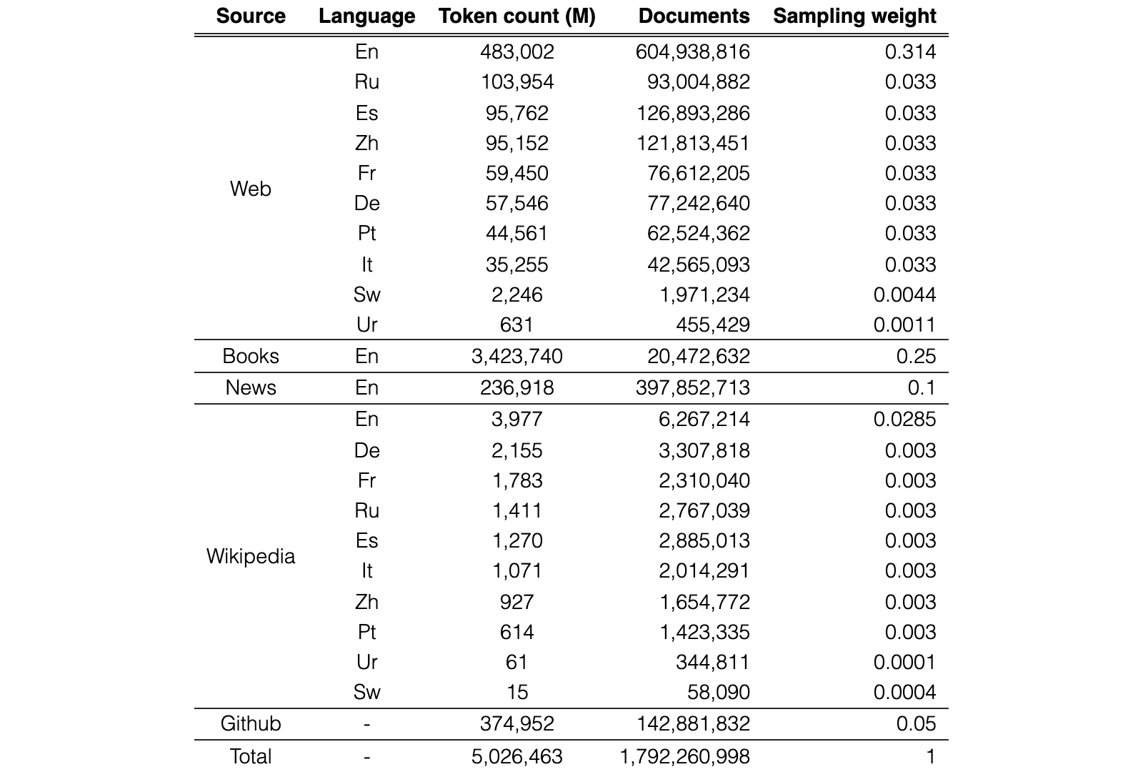
The full break down of MassiveText by source and languages is given in Table 8. For a full description and analysis of MassiveText, see Rae et al. (2021).
| Source | Language | Token count (M) | Documents | Sampling weight |
|---|---|---|---|---|
| Web | En | 483,002 | 604,938,816 | 0.314 |
| Ru | 103,954 | 93,004,882 | 0.033 | |
| Es | 95,762 | 126,893,286 | 0.033 | |
| Zh | 95,152 | 121,813,451 | 0.033 | |
| Fr | 59,450 | 76,612,205 | 0.033 | |
| De | 57,546 | 77,242,640 | 0.033 | |
| Pt | 44,561 | 62,524,362 | 0.033 | |
| It | 35,255 | 42,565,093 | 0.033 | |
| Sw | 2,246 | 1,971,234 | 0.0044 | |
| Ur | 631 | 455,429 | 0.0011 | |
| Books | En | 3,423,740 | 20,472,632 | 0.25 |
| News | En | 236,918 | 397,852,713 | 0.1 |
| Wikipedia | En | 3,977 | 6,267,214 | 0.0285 |
| De | 2,155 | 3,307,818 | 0.003 | |
| Fr | 1,783 | 2,310,040 | 0.003 | |
| Ru | 1,411 | 2,767,039 | 0.003 | |
| Es | 1,270 | 2,885,013 | 0.003 | |
| It | 1,071 | 2,014,291 | 0.003 | |
| Zh | 927 | 1,654,772 | 0.003 | |
| Pt | 614 | 1,423,335 | 0.003 | |
| Ur | 61 | 344,811 | 0.0001 | |
| Sw | 15 | 58,090 | 0.0004 | |
| Github | - | 374,952 | 142,881,832 | 0.05 |
| Total | - | 5,026,463 | 1,792,260,998 | 1 |
View original table
| Megan Rohrer | Aakashavaani |
| Emma Raducanu | Junior Eurovision Song Contest 2021 |
| Ambra Sabatini | Pavilion Bukit Jalil |
| WhyDonate | Blake Desjarlais |
| The Juggernaut (company) | 2021 All-Ireland Senior Football Championship Final |
| Angela Diaz | Drift-barrier hypothesis |
| 2020 Summer Paralympics | Venomics |
| 2021 Afghan protests | Great Circle (novel) |
| Rexh Xhakli | Hurricane Ida |
| Julia Laskin | 2021 Montenegrin episcopal enthronement protests |
| Cuijk | At War With the Silverfish |
| Ghoubet Wind Power Station |
View original table
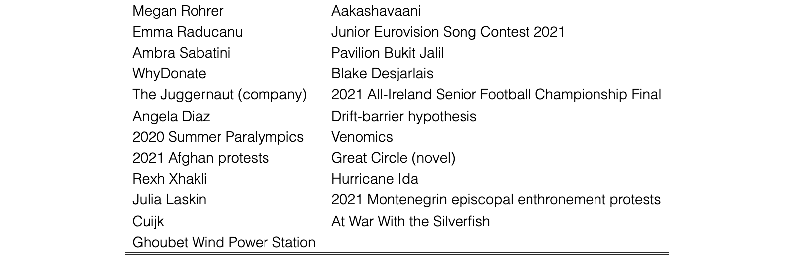
We create an evaluation dataset consisting of 23 Wikipedia articles that were added or heavily edited in September 2021, after we collected our training dataset. In addition, we filter out articles that rely too heavily on templated content, using the method detailed in §2.6 to identify articles with chunks that have a high overlap with their neighbours. Fig. 10 show that little overlap remains between our test dataset and the retrieved neighbours from the training dataset. The full list of included articles is given in Table 9.
We first parse articles using mwparserfromhell. We then remove sections with the following titles: “references”, “external links”, “sources”, “further reading”, “see also”, “citations”, and “note”. In the remaining sections, we remove Wikilinks and remove the following templates: “reflist”, “notelist”, “notelist-ua”, “notelist-lr”, “notelist-ur”, and “notelist-lg”. We also exclude objects with the “ref” or “table” tag and clean the remaining text with the strip_code function. Finally, we concatenate the title and all the sections and use \n\n to delimitate them.
We give details on the Retro architecture, and on the fine-tuning procedure we use for Retrofitting existing language models.
As mentioned in the main text, the overall encoder-decoder architecture is fully feed-forward. We start with a sequence , and its pre-computed neighbours and returns logits in . Along with Attn, Ffw, Cca and Ca operators introduced in the main text, we define the decoder embedding layer , the Split operator that extracts chunked intermediary embeddings and the read-out layer . We then describe the forward pass in Algorithm 1. In addition to the usual Transformer ones, Retro architecture hyperparameters involves the layer indices and , at which the encoder and the decoder perform cross-attention.
The Ca operator uses relative positional logits, that are computed from a specific relative distance separating data tokens from retrieval tokens. Indeed, we expect any retrieval neighbour and the chunk to be relatively well aligned, and assume that they start at the same position. Therefore, when computing , we set the distance between the data token of chunk and the retrieval token of to be
When computing the encoder cross-attentions , we set the distance between the retrieval token and the data token to be
Positional logits are obtained as a linear transform of a cosine vector computed from , and are added to content logits, as in a regular self-attention block.
Our implementation of the Cca operator, shown in 1, is based on a vectorized application of a cross-attention layer. For simplicity, we omit the multi-head attention logic and use the simplest Q,K,V attention. We omit relative positional logits computation, described above.
We use disjoint embeddings for the encoder and decoder by default, which allows us to use a different dimensionality for the encoder (typically kept at and for the decoder (that we scale up to ). It is possible to share the embeddings, with little difference in training, as we show in the ablation section.
As shown in Fig. 5, we found that we were able to take a pre-trained baseline transformer and add Retro through fine-tuning. In all cases, we froze all weights from pre-training and freshly initialised the retrieval encoder and cross-attention weights. In all cases, the cross-attention is added every third layer starting at layer six. The learning rate for the three smaller models was set to and half that for the larger model. We experimented with allowing the entire model to resume training during fine-tuning but consistently found that the best approach was to freeze the pre-trained model. This kept the retrieval-off performance frozen whereas when all weights were tuned the retrieval off performance would degrade.
We provide the hyperparameters used in the various experiments of §4.
In Table 10, we show the hyperparameters of the different models we train. In all cases, we train for 419,430,400,000 training tokens. The three smaller models are trained with a batch size of 256 and the largest model is trained with a batch size of 1024. The minimum learning rate is set to 0.1 times the maximum learning rate, which is shown in Table 10. The learning rate is decayed using a cosine cycle length that matches the total number of training tokens. All models are trained using AdamW (Loshchilov and Hutter, 2019) with a weight decay parameter of 0.1. The learning rate linearly increases from to the maximum learning rate over the first 750 steps of training.
| Baseline | heads | Head size | layers | Max LR | ||||
|---|---|---|---|---|---|---|---|---|
| 247M | 896 | 3584 | 16 | 64 | 12 | 2 | ||
| 564M | 1536 | 6144 | 12 | 128 | 12 | 2 | ||
| 1,574M | 2048 | 8192 | 16 | 128 | 24 | 2 | ||
| 7,505M | 4096 | 16384 | 32 | 128 | 32 | 1 |
View original table

All models use ZeRO to shard the optimiser state (Rajbhandari et al., 2020). Additional infrastructure details can be found in Rae et al. (2021).
| Model | Number of layers | 18 |
| 1024 | ||
| 4096 | ||
| Key size | 64 | |
| Value size | 64 | |
| Number of heads | 16 | |
| Training data | Dataset | Wikitext103train |
| Sequence length | 3072 | |
| Batch size | 128 | |
| Tokenizer vocabulary size | 128,000 | |
| Optimisation | optimiser | Adam |
| Adam’s | 0.9 | |
| Adam’s | 0.95 | |
| Adam’s | 1e-8 | |
| Dropout rate | 0.25 | |
| Schedule | Learning rate start | 1e-7 |
| Learning rate max | 2.5e-4 | |
| Learning rate min | 2e-5 | |
| Warmup steps | 4,000 | |
| Cosine cycle steps | 100,000 | |
| Evaluation | Overlapping proportion | 87.5 % |
View original table
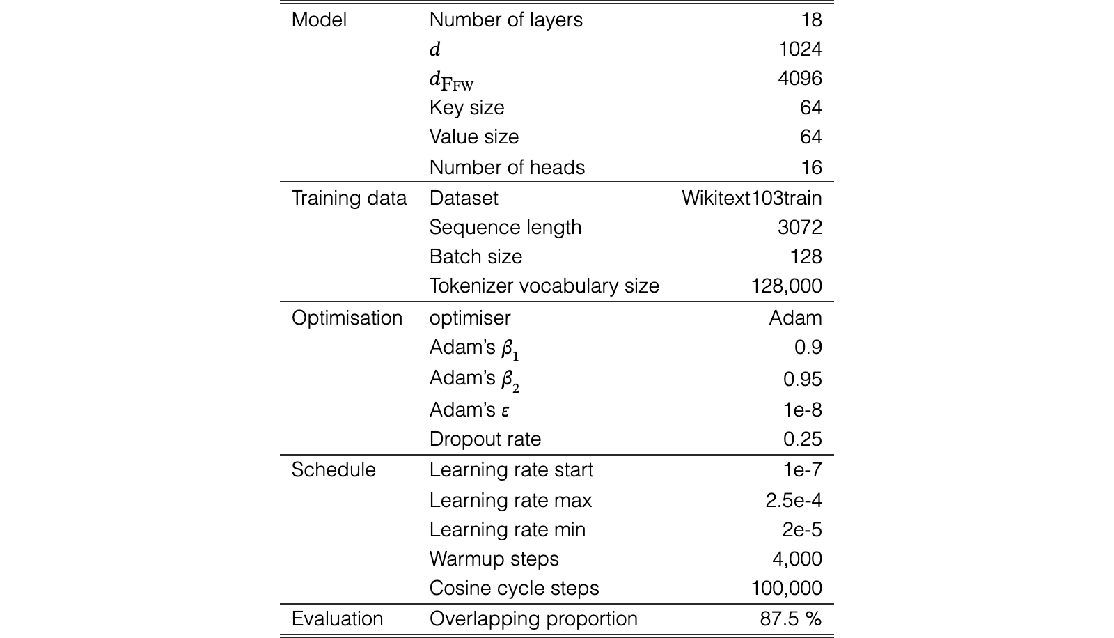
We provide more details on our Wikitext103 results presented in §4.1 and Table 4. We train a baseline transformer on the Wikitext103 training set with the hyperparameters presented in Table 11. The learning rate ramps linearly from to in the first 4,000 steps, then decays to at 100,000 steps using a cosine schedule. The baseline checkpoint at step 35,000 has the lowest perplexity on Wikitext103 valid, of , for overlapping proportion of 75% (sliding window evaluation that only uses probabilities for tokens that have at least 75% of the sequence length of context, when available). We use this checkpoint for all our baseline and numbers reported in Table 4, except that Table 4 reports for an overlapping proportion of 87.5 %, which slightly lowers the perplexity of our baseline to 21.53 on Wikitext103 valid.
We also use the 35,000 step baseline checkpoint as initialization for a Retrofit, which otherwise uses the same optimiser and schedule hyperparameters but only trains the new retrieval weights, as explained in §4.2. Our best Retrofit checkpoint has a Wikitext103 valid perplexity , when retrieving from Wikipedia. We use this Retro checkpoint in Table 4 for all other retrieval sets. The evaluation curves for our baseline and Retrofit is shown if Fig. 7 (left). In this particular case, because Wikitext103 is quite small, training a Retro model from scratch led to weaker results than the baseline, at least when retrieving from Wikipedia, as we couldn’t find an effective way to mitigate the increased over-fitting due to the additional weights of Retro.
We also re-implement using the same tokenizer and dataset that we use for our baseline and Retrofitting experiments. has probabilities with . To tune and , we begin with , which corresponds to the inverse of the standard deviation of the norm of the embeddings that we use as keys and queries for . We find the best . We then find the best for that value of . Fig. 7 center and right respectively show the perplexity of as a function of and .
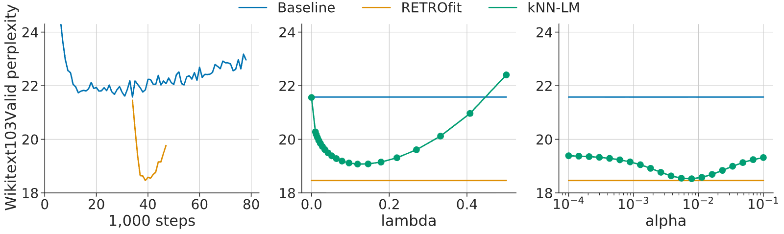
In Table 12, we give the hyperparameters used for Retrofitting the models on Massive Text.
| Model | Layers with Retro-block () | Learning rate | Batch size |
|---|---|---|---|
| 172M | Every 3 from 6 | 256 | |
| 425M | Every 3 from 6 | 256 | |
| 1.5B | Every 3 from 6 | 256 | |
| 7.5B | Every 3 from 6 | 256 |
View original table

We fine-tune our 7.5B Retro model for 25,000 steps, using a batch size of 128, a learning rate cosine scheduled from to , with a linear ramp of 750 steps. We use dropout in the decoder only, as it performs better than using dropout in both the encoder and the decoder. Each neighbour is formatted as title: {title}, source: {source}. We use the top 20 neighbours from Dpr when training and evaluating.
| Ablation group | Ablation | C4 eval bpb |
| Model | Retro | 0.822 |
| No query conditioning | 0.829 | |
| No CA positional encodings | 0.826 | |
| Shared embeddings | 0.823 | |
| 6-layer encoder | 0.821 | |
| Retrieval values | Neighbours N | 0.950 |
| Continuations F | 0.895 | |
| No retrieval | 0.987 | |
| Training neighbours | 1 training neighbours | 0.858 |
| 4 training neighbours | 0.847 | |
| Cross attention position | CA top layer (1/12) | 0.827 |
| CA mid layer (6/12) | 0.823 | |
| CA top layer (12/12) | 0.831 | |
| CA all layers | 0.860 | |
| CA every 3 from 1 | 0.823 |
View original table
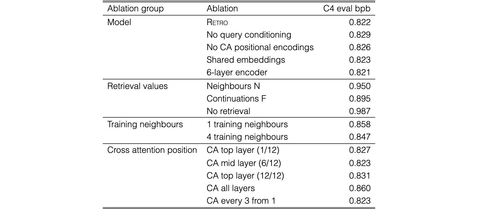
We validate important design choices by evaluating what happens when we do not include them. We use the 247M parameter model for all experiments and we train on a compressed 157 billion token schedule for all ablation experiments. We describe results relative to the default settings presented in the main text and recalled here. We report C4 evaluation loss at the end of the training process, and also compares how the evaluation loss decrease versus the training time, measured relatively to the baseline training time. Results are reported in Fig. 8 and Table 13.
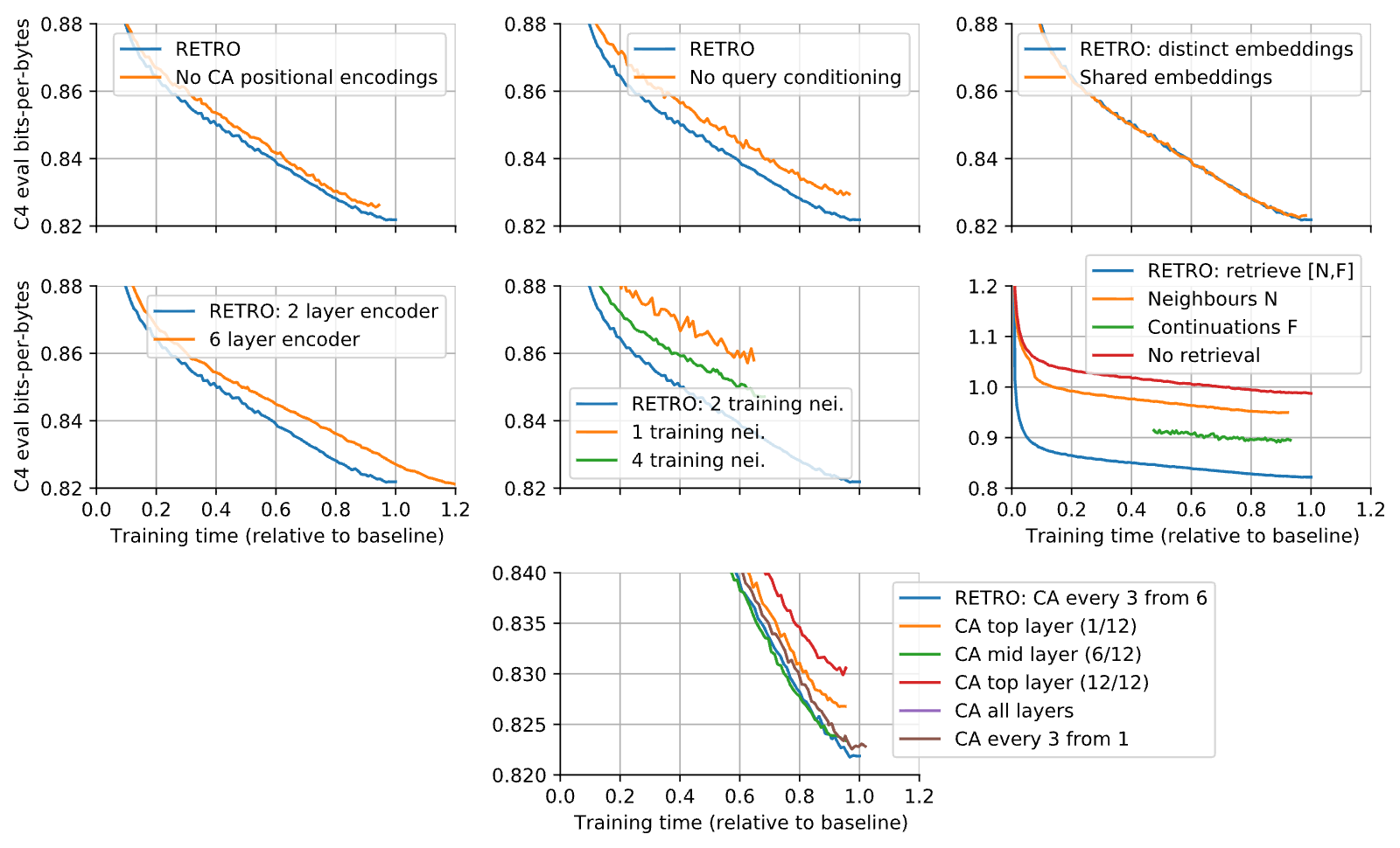
Using relative encodings in cross-attention, as described in §B.1.2, provides a pure improvement both in the number of steps to reach a given performance and computational efficiency.
Conditioning the encoder on the previous chunk’s intermediate embeddings, as described in §B.1.1, provides a pure improvement both in term of number of steps and computational efficiency.
Sharing embeddings across the encoder and the decoder does not affect performance. This motivates us using separate embeddings, as it allows to have a narrower encoder than decoder as we scale up the decoder size.
Retro models are trained by attending, for a given chunk, to both the neighbours of the preceding chunk and their continuation in time. We measure how training and evaluating Retro models on neighbours only and their continuation only affects performance. Overall, attending to neighbours only provides of the performance improvement due to retrieval in Retro, while attending the future of the neighbours gives of the performance. Attending to both neighbours and their continuation is the most efficient choice both in term of final performance and training efficiency.
All models in the text use a relatively small Retro encoder. We experimented with a deeper encoder. We found that this resulted in a tiny decrease in loss– 0.15% at the cost of a larger training time (). Overall, using a shallow encoder is the best choice in term of training efficiency.
We measure the effect of training on a single retrieved neighbour, as well as training on 4 neighbours (Retro uses 2 neighbours in training). Training on a single neighbour results in a large decrease in performance, while training on 4 neighbours does not give substantial performance improvement at the end of training, but induces a large computational overhead. Overall, we find that using 2 neighbours is the best choice in term of training efficiency. Furthermore, evaluation can be done with additional neighbours.
We measure how the frequency of cross-attention in the decoder affects performance. Overall, attending only once at the top or the bottom layer is a bad choice, while attending once on a mid-depth layer is relatively sound. We choose to have cross-attention every 3 layer as this provides a good trade-off between performance and run-time.
We illustrate the usage of Retro models by looking at the perplexity of evaluation samples and by producing samples autoregressively.
To build an intuition of what kind of information is leveraged by Retro models, we suggest to have a closer look at a few evaluation documents and the corresponding retrieved data in Tables 16, 17, 18 and 19. In these tables, the 4 rows corresponds to the first 4 chunks of the documents. The left-most column shows the chunk from the document being evaluated, where each token is coloured by the negative cross entropy loss difference , a positive value, coloured in yellow, indicates that Retro performs better when it has access to neighbours data. The second columns also shows the evaluated chunk but where each token is coloured by the length of the longest common prefix (LCP) with the preceding neighbours, i.e. the largest integer such that the prefix also appears in . Conversely, columns three and four show the first two neighbours and their continuation, respectively and coloured by LCP with subsequent chunk . LCP colouring helps to visually identify where the evaluated document overlaps the retrieved data. Note that the first chunk, , in the second column is not coloured as it does not have any preceding neighbours to compute LCP with. Similarly, we do not show the neighbours of the fourth chunk, as these are not used to condition any of the first four chunks.
Our qualitative analysis exhibits two major behaviors.
Firstly, we observe that sometimes, specific facts in can be extracted from the preceding neighbours and that this can correspond to significant reduction in loss from the Retro model for the corresponding tokens. Some examples of such behavior include the journal name Publishers Weekly in Table 16, the football team name Tyrone in Table 17 or the event dates 25 August to 6 September 2020 in Table 18. In these three examples, the evaluated data consists of recent Wikipedia articles written in September 2021, after we built our retrieval dataset (see section §A.2). Yet, relevant information to predict this new data was available in the pre-existing retrieval data and the Retro model seems to be able to correctly leverage it.
On the other hand, we also observe that some of the evaluation data can partially leak in our training and retrieval data, despite the use of deduplication. Retro can dramatically exploit such leakage. Table 19 illustrates this behavior, where the chunks and largely overlaps and respectively, up to small formatting differences, which leads to much lower Retro loss for all the corresponding tokens. Fig. 6 shows that it is possible to quantify how much of the Retro loss reduction is due to each of these two behaviors, by filtering out evaluation chunks that overlaps with the retrieval set.
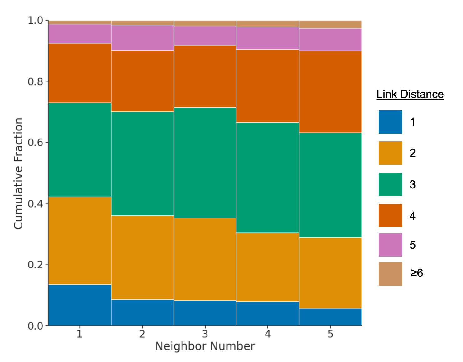
To quantify a notion of distance between the source document and the retrieved chunks, we can ask the distance between source articles when retrieving only from Wikipedia. Consonni et al. (2019) provides a Wikipedia link dataset which, for each article, contains a list of neighbouring articles. Using this, we construct a directed graph and compute the distance from one page to another. In Fig. 9 we compute the link-distance between training sequences and the retrieved neighbours. We find that retrieved documents tend to be from articles that are quite close to the article containing the target. Furthermore, we find that on average the distance increases with rank, suggesting that our neighbours are both useful and that the order is reasonable. This provides confidence for our larger-scale experiments where document distance is less well defined.
We report tables corresponding to quantitative figures of the main text, as well as further filtered language model results on the Pile.
We report the performance of Retro and baseline models, measured in bits-per-bytes on evaluation set, in Table 14.
| Baseline | Retro [Off] | Retro[On] | ||||||||||
| 172M | 425M | 1.5B | 7.5B | 172M | 425M | 1.5B | 7.5B | 172M | 425M | 1.5B | 7.5B | |
| C4 Eval bpb | 0.98 | 0.92 | 0.84 | 0.78 | 0.98 | 0.92 | 0.84 | 0.78 | 0.82 | 0.77 | 0.71 | 0.66 |
| C4 Eval bpb (900B) | - | - | - | - | - | - | - | - | 0.88 | 0.83 | 0.76 | 0.71 |
| C4 Eval bpb (360B) | - | - | - | - | - | - | - | - | 0.92 | 0.87 | 0.80 | 0.74 |
| C4 Eval bpb (180B) | - | - | - | - | - | - | - | - | 0.94 | 0.89 | 0.81 | 0.75 |
| C4 Eval bpb (90B) | - | - | - | - | - | - | - | - | 0.95 | 0.89 | 0.82 | 0.76 |
| C4 Eval bpb (36B) | - | - | - | - | - | - | - | - | 0.96 | 0.90 | 0.83 | 0.77 |
| C4 Eval bpb (18B) | - | - | - | - | - | - | - | - | 0.96 | 0.91 | 0.83 | 0.77 |
| C4 Eval bpb (9B) | - | - | - | - | - | - | - | - | 0.96 | 0.91 | 0.83 | 0.77 |
| C4 Eval bpb (4B) | - | - | - | - | - | - | - | - | 0.97 | 0.91 | 0.84 | 0.78 |
| C4 Eval bpb (2B) | - | - | - | - | - | - | - | - | 0.97 | 0.91 | 0.84 | 0.78 |
| C4 Eval bpb () | - | - | - | - | - | - | - | - | 0.84 | 0.79 | 0.73 | 0.67 |
| C4 Eval bpb () | - | - | - | - | - | - | - | - | 0.83 | 0.78 | 0.72 | 0.67 |
| C4 Eval bpb () | - | - | - | - | - | - | - | - | 0.82 | 0.78 | 0.71 | 0.66 |
| C4 Eval bpb () | - | - | - | - | - | - | - | - | 0.82 | 0.77 | 0.71 | 0.66 |
| C4 Eval bpb () | - | - | - | - | - | - | - | - | 0.82 | 0.77 | 0.71 | 0.66 |
| C4 Eval bpb () | - | - | - | - | - | - | - | - | 0.82 | 0.77 | 0.71 | 0.66 |
| C4 Eval bpb () | - | - | - | - | - | - | - | - | 0.82 | 0.77 | 0.71 | 0.66 |
| C4 Eval bpb () | - | - | - | - | - | - | - | - | 0.82 | 0.77 | 0.71 | 0.65 |
| C4 Eval bpb () | - | - | - | - | - | - | - | - | 0.83 | 0.77 | 0.71 | 0.65 |
| C4 Eval bpb () | - | - | - | - | - | - | - | - | 0.83 | 0.78 | 0.71 | 0.66 |
| C4 Eval bpb () | - | - | - | - | - | - | - | - | 0.84 | 0.78 | 0.72 | 0.66 |
| C4 Eval bpb () | - | - | - | - | - | - | - | - | 0.84 | 0.79 | 0.72 | 0.66 |
| C4 Eval bpb () | - | - | - | - | - | - | - | - | 0.85 | 0.79 | 0.73 | 0.66 |
| C4 Eval bpb () | - | - | - | - | - | - | - | - | 0.85 | 0.79 | 0.73 | 0.66 |
| C4 Eval bpb () | - | - | - | - | - | - | - | - | 0.85 | 0.79 | - | 0.67 |
| Lambada Accuracy | 0.42 | 0.51 | 0.61 | 0.69 | 0.47 | 0.54 | 0.63 | 0.70 | 0.52 | 0.60 | 0.67 | 0.73 |
| Curation Corpus bpb | 0.69 | 0.63 | 0.56 | 0.52 | 0.68 | 0.64 | 0.57 | 0.51 | 0.66 | 0.61 | 0.55 | 0.50 |
| Wikitext103 Perplexity | 25.62 | 19.29 | 13.98 | 10.65 | 25.88 | 19.78 | 13.89 | 10.40 | 3.32 | 2.96 | 2.53 | 2.22 |
| Wikipedia Sept. 2021 bpb | 0.85 | 0.78 | 0.71 | 0.65 | 0.86 | 0.79 | 0.71 | 0.65 | 0.79 | 0.73 | 0.66 | 0.61 |
View original table
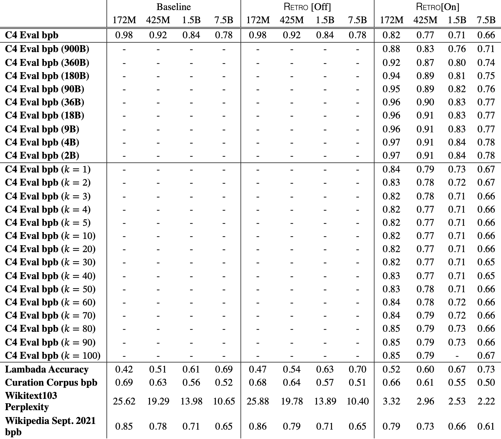
In Fig. 4, we compare Retro against Jurassic-1 (Lieber et al., 2021). The full bits-per-bytes results are reported in Table 15.
| Subset | 7B Baseline (Ours) | GPT-3 | Jurassic-1 | Gopher | 7.5B Retro |
|---|---|---|---|---|---|
| arxiv | 0.742 | 0.838 | 0.680 | 0.641 | 0.714 |
| books3 | 0.792 | 0.802 | 0.835 | 0.706 | 0.653 |
| dm_mathematics | 1.177 | 1.371 | 1.037 | 1.135 | 1.164 |
| freelaw | 0.576 | 0.612 | 0.514 | 0.506 | 0.499 |
| github | 0.420 | 0.645 | 0.358 | 0.367 | 0.199 |
| gutenberg_pg_19 | 0.803 | 1.163 | 0.890 | 0.652 | 0.400 |
| hackernews | 0.971 | 0.975 | 0.869 | 0.888 | 0.860 |
| nih_exporter | 0.650 | 0.612 | 0.590 | 0.590 | 0.635 |
| opensubtitles | 0.974 | 0.932 | 0.879 | 0.894 | 0.930 |
| philpapers | 0.760 | 0.723 | 0.742 | 0.682 | 0.699 |
| pile_cc | 0.771 | 0.698 | 0.669 | 0.688 | 0.626 |
| pubmed_abstracts | 0.639 | 0.625 | 0.587 | 0.578 | 0.542 |
| pubmed_central | 0.588 | 0.690 | 0.579 | 0.512 | 0.419 |
| stackexchange | 0.714 | 0.773 | 0.655 | 0.638 | 0.624 |
| ubuntu_irc | 1.200 | 0.946 | 0.857 | 1.081 | 1.178 |
| uspto_backgrounds | 0.603 | 0.566 | 0.537 | 0.545 | 0.583 |
View original table
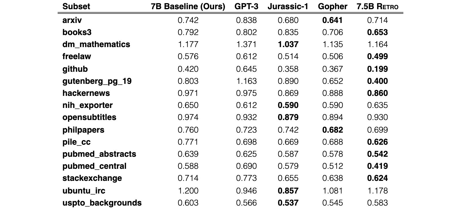
We evaluate leakage between the evaluation sets and the training set by measuring the proportion of evaluation chunks with a certain overlap . We show histograms in Fig. 10. We can see that has some slight overlaps between train and evaluation. Similarly, chunks of Wikitext103 appear in the training set despite having removed the actual Wikitext103 evaluation documents from the training set. On the other hand, our Wikipedia September 21 dataset shows almost no leakage (data being original documents that did not exist at training data creation), and neither does Curation Corpus.
We report chunk overlap distribution and filtered performance curves on the Pile in Fig. 12 and Fig. 11, respectively. The qualitative interpretation of the filtered curves is the same: Retro models exploit leakage more, but the performance improvement they provide remains significant even on original chunks that haven’t been observed in the training set.
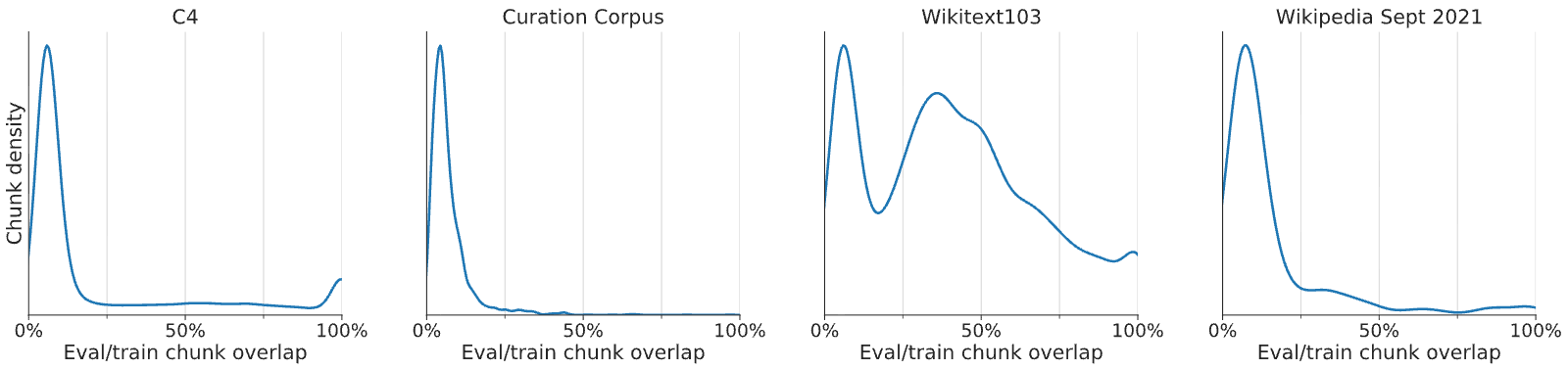
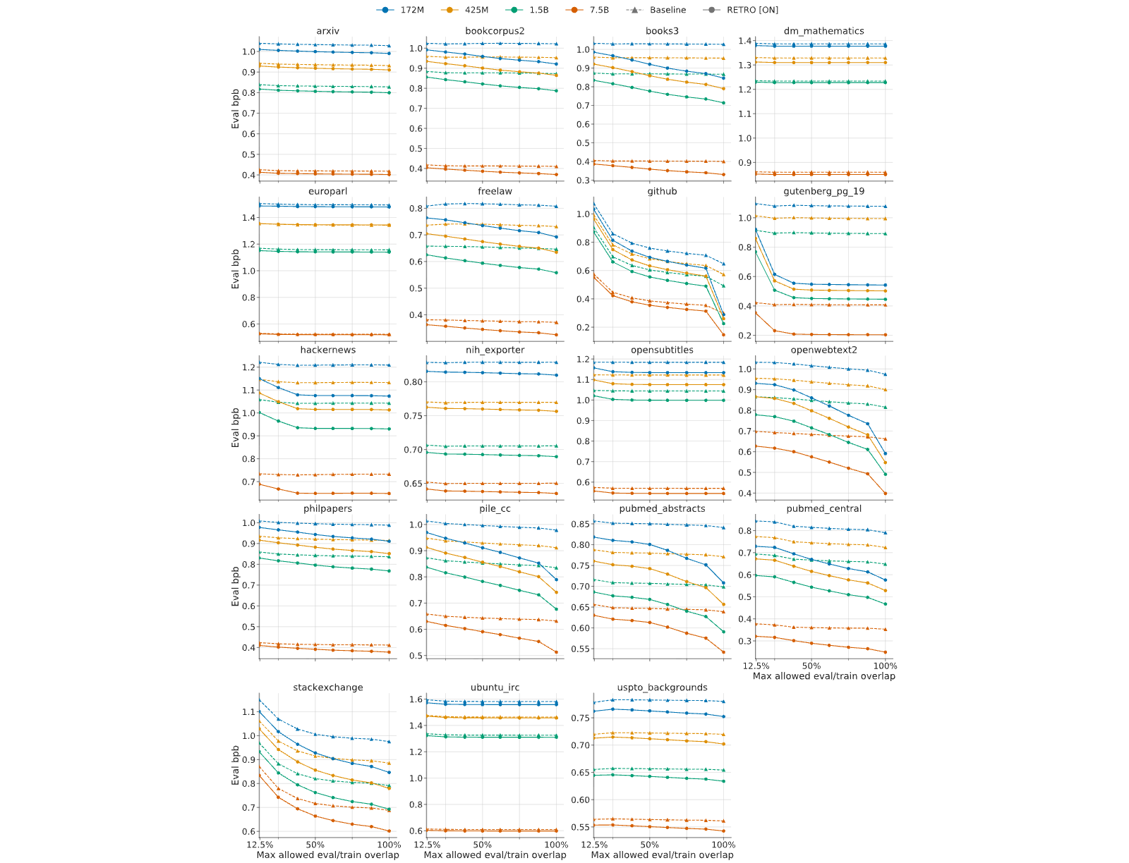
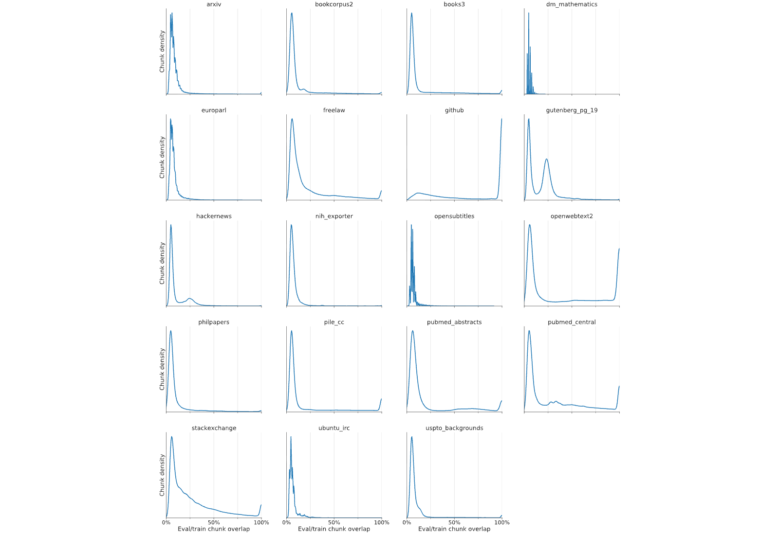
| colored by loss difference | colored by LCP with | colored by LCP with | colored by LCP with |
L_{\textsc{{Retro[Off]} }}-L_{\textsc{Retro}}\hbox{\pagecolor{cm_0!40}\leqslant-0.5},\hbox{\pagecolor{cm_31!40}=0},\hbox{\pagecolor{cm_63!40}\geqslant 0.5} | , , , ,, | , , , ,, | , , , ,, |
| Great Circle (novel)Great Circle i | Great Circle (novel) Great Circle i | The Dutch House (novel)The Dutch H | The Dutch House (novel)The Dutch H |
| s a 2021 novel by Maggie Shipstead, | s a 2021 novel by Maggie Shipstead, | ouse is a 2019 novel by Ann Patchett | ouse is a 2019 novel by Ann Patchett |
| published on May 4, 2021, by Alfred | published on May 4, 2021, by Alfred | . It was published by Harper on Sept | . It was published by Harper on Sept |
| A. Knopf.The novel has been shortl | A. Knopf. The novel has been shortl | ember 24, 2019. It tells the story o | ember 24, 2019. It tells the story o |
| isted for the 2021 Booker Prize.Sy | isted for the 2021 Booker Prize. Sy | f a brother and sister over the cour | f a brother and sister over the cour |
| nopsis The novel consists of two pa | nopsis The novel consists of two pa | se of five decades.The novel was a | se of five decades.[2]The novel wa |
| rallel narratives about two fictiona | rallel narratives about two fictiona | finalist for the 2020 Pulitzer Priz | s a finalist for the 2020 Pulitzer P |
| l women. One is | l women. One is | e for Fiction.PlotThe Dutch House | rize for Fiction.[3]Plot[edit]Th |
| is a mansion located in Elkins Park | e Dutch House is a mansion located i | ||
| , Pennsylvania, a suburb of Philadel | n Elkins Park, Pennsylvania, a subur | ||
| phia. It was built in 1922 by the Va | b of Philadelphia. It was built in 1 | ||
| nHoebeek family, a husband and wife | 922 by the VanHoebeek family, a husb | ||
| originally from the Netherlands who | and and wife originally from the Net | ||
| made their fortune in the tobacco in | herlands who made their fortune in t | ||
| dustry. Cyril Conroy, a self-made re | he tobacco industry. Cyril Conroy, a | ||
| al estate mogul | self- | ||
| about the disappeared 20th-century | about the disappeared 20th-century | on becoming a filmmaker. She has fo | based closely on her own youthful e |
| aviator Marian Graves, while the oth | aviator Marian Graves, while the oth | und a subject for her film project, | xperiences. (She plans the film to b |
| er is about the struggling 21st-cent | er is about the struggling 21st-cent | an obscure African American actress | e the first of two parts, the second |
| ury Hollywood actress Hadley Baxter, | ury Hollywood actress Hadley Baxter, | credited only as “the watermelon wom | dealing with the aftermath of the f |
| who is attempting to make a film ab | who is attempting to make a film ab | an” in old Hollywood films, and the | irst’s events.) Byrne plays a young |
| out Marian. Hadley’s narrative is to | out Marian. Hadley’s narrative is to | subsequent film recounts her search | film student named Julie (Hogg’s ava |
| ld in the first-person, while Marian | ld in the first-person, while Marian | for this woman even as it covers, in | tar), who starts her artistic educat |
| ’s sections are told in the third-pe | ’s sections are told in the third-pe | the manner of the earlier Dunyement | ion with high hopes of making a movi |
| rson | rson | aries, Dunye’s friendships and her l | e about a boy named Tony, living in |
| ove life. InThe Watermelon Woman, D | working-class Sunderland, who adores | ||
| unye makes the film she set out to m | his mother — “is almost obsessed wi | ||
| ake in 1990 about African American w | th her,” as eager Julie tells her ad | ||
| omen artists, a film that both inven | visers. Her idealism is evident from | ||
| ts an artistic predecessor with whom | the start.The advisers are skepti | ||
| she can identify and also “finds” C | cal, and no wonder; Julie’s family i | ||
| heryl herself as the artist that she | s posh, with a comfortable country e | ||
| seeks. As Dunye identifies herself | state and | ||
| .Reception Great Circle received | .Reception Great Circle received | first edition hardcoverReception | The book also debuted at number tw |
| very favorable reviews, with a cumul | very favorable reviews, with a cumul | The novel debuted at number one on T | o on The New York Times Hardcover No |
| ative "Rave" rating at the review ag | ative "Rave" rating at the review ag | he New York Times fiction best-selle | nfiction best-sellers list on July 2 |
| gregator website Book Marks, based o | gregator website Book Marks, based o | r list. As of the week ending Februa | 8, 2019.[5] It spent eleven weeks on |
| n 22 book reviews from mainstream li | n 22 book reviews from mainstream li | ry 20, 2021, the novel has spent 38 | the list.[6]Reception[edit]At t |
| terary critics. The novel debuted at | terary critics. The novel debuted at | weeks on the list.At the review ag | he review aggregator website Book Ma |
| number fourteen on The New York Tim | number fourteen on The New York Tim | gregator website Book Marks, which a | rks, which assigns individual rating |
| es Hardcover fiction best-seller lis | es Hardcover fiction best-seller lis | ssigns individual ratings to book re | s to book reviews from mainstream li |
| t for the week ending May | t for the week ending May | views from mainstream literary criti | terary critics, the book received a |
| cs, the novel received a cumulative | cumulative "Positive" rating based o | ||
| "Rave" rating based on 38 reviews, w | n 29 reviews: 12 "Rave" reviews, 6 " | ||
| ith only one "mixed" review. Publish | Positive" reviews, 9 "Mixed" reviews | ||
| ers Weekly wrote, "Bennett renders h | , and 2 "Pan" reviews.[7]Publisher | ||
| er characters and their struggles wi | s Weekly gave the book a mixed revie | ||
| th great compassion, and explores th | w, writing, "Unfortunately, all thre | ||
| e complicated state of mind that Ste | e | ||
| lla finds herself in while passing a | |||
| s white." In its | |||
| 8, 2021. Critics praised the novel | 8, 2021. Critics praised the novel | ||
| for sustaining its length and for Sh | for sustaining its length and for Sh | ||
| ipstead’s research and intricate nov | ipstead’s research and intricate nov | ||
| el structure for perfectly interweav | el structure for perfectly interweav | ||
| ing the parallel narratives, despite | ing the parallel narratives, despite | ||
| the time and circumstances separati | the time and circumstances separati | ||
| ng them.In its starred review, Pub | ng them.In its starred review, Pub | ||
| lishers Weekly wrote, "Shipstead man | lishers Weekly wrote, "Shipstead man | ||
| ages to portray both Marian’s and Ha | ages to portray both Marian’s and Ha | ||
| dley’s | dley’s |
View original table
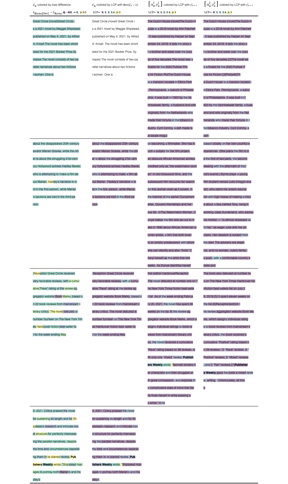
| colored by loss difference | colored by LCP with | colored by LCP with | colored by LCP with |
L_{\textsc{{Retro[Off]} }}-L_{\textsc{Retro}}\hbox{\pagecolor{cm_0!40}\leqslant-0.5},\hbox{\pagecolor{cm_31!40}=0},\hbox{\pagecolor{cm_63!40}\geqslant 0.5} | , , , ,, | , , , ,, | , , , ,, |
| 2021 All-Ireland Senior Football Cha | 2021 All-Ireland Senior Football Cha | 2018 All-Ireland Senior Football Cha | 2018 All-Ireland Senior Football Cha |
| mpionship FinalThe 2021 All-Irelan | mpionship Final The 2021 All-Irelan | mpionship FinalThe 2018 All-Irelan | mpionship FinalThe 2018 All-Irelan |
| d Senior Football Championship Final | d Senior Football Championship Final | d Senior Football Championship Final | d Senior Football Championship Final |
| was the 134th final of the All-Irel | was the 134th final of the All-Irel | was the 131st final of the All-Irel | was the 131st final of the All-Irel |
| and Senior Football Championship and | and Senior Football Championship and | and Senior Football Championship and | and Senior Football Championship and |
| the culmination of the 2021 All-Ire | the culmination of the 2021 All-Ire | the culmination of the 2018 All-Ire | the culmination of the 2018 All-Ire |
| land Senior Football Championship. T | land Senior Football Championship. T | land Senior Football Championship in | land Senior Football Championship in |
| he match was played at Croke Park in | he match was played at Croke Park in | Gaelic football. The match was play | Gaelic football. The match was play |
| Dublin on 11 September 2021. It was | Dublin on 11 September 2021. It was | ed at Croke Park in Dublin on 2 Sept | ed at Croke Park in Dublin on 2 Sept |
| originally scheduled | originally scheduled | ember 2018.[3]It was the second ti | ember 2018.It was the second time |
| me the teams had met in the final; D | the teams had met in the final; Dubl | ||
| ublin won the first encounter in 199 | in won the first encounter in 1995. | ||
| 5.The final was shown live in Irel | It was the third consecutive year th | ||
| and on RTÉ Two as part of The Sunday | at a team qualified under the system | ||
| Game live programme, presented by M | of second chances introduced in 200 | ||
| ichael Lyster from Croke Park, with | 1; Tyrone qualified despite defeat i | ||
| studio analysis from Joe Brolly, | n its provincial championship.Dubl | ||
| in won the final by a margin of six | |||
| points | |||
| for 28 August but had to be postpon | for 28 August but had to be postpon | game 23–23 after extra time, howeve | with a last-ditch plan of action – |
| ed by two weeks when the – semi-fina | ed by two weeks when the – semi-fina | r Ulster progressed under the compet | play the Munster/Ulster Semi-Final o |
| l was postponed due to a COVID-19 ou | l was postponed due to a COVID-19 ou | ition rules as they scored three tir | n March 16th, with the winners to pl |
| tbreak. Ulster champions Tyrone took | tbreak. Ulster champions Tyrone took | es in the match against Leinster’s t | ay Connacht in the following day’s F |
| on Connacht champions Mayo, in what | on Connacht champions Mayo, in what | wo. The semi-finals took place in mi | inal.On March 16th then Munster ha |
| was their first ever meeting in a f | was their first ever meeting in a f | d November and saw both the away tea | d an easy win over Ulster (9-07 to 0 |
| inal, winning their 4th title after | inal, winning their 4th title after | ms win, as Ulster beat Glasgow and E | -00) but thankfully for the Munster |
| a 2–14 to 0–15 win. Mayo lost | a 2–14 to 0–15 win. Mayo lost | dinburgh beat Connacht. The final wa | players, the pitch cut up so badly d |
| s held on Saturday December 20 at Mu | uring the game, it was decided to po | ||
| rrayfield Stadium and saw Ulster bea | stpone the following day’s hurling F | ||
| t Edinburgh 21–27 to win the Celtic | inal (until Easter Sunday) with the | ||
| Cup.2004–05 seasonThe format of | football Final going ahead on its ow | ||
| the competition was changed for the | n on St. Patrick’s Day.Less than a | ||
| second edition of the competition. T | week later, on March 23rd, seven | ||
| he competition was moved to April an | |||
| d May to run after the conclusion of | |||
| the Celtic League competition, with | |||
| only eight | |||
| their 11th consecutive final since | their 11th consecutive final since | 1-16 to 0-15 winners to qualify for | which Dublin won by 0-12 to 0-9.D |
| 1989, losing 6 finals in 9 years, wi | 1989, losing 6 finals in 9 years, wi | their 10th league final in the past | ublin are going for an unprecedented |
| th this latest defeat on an identica | th this latest defeat on an identica | 13 years.They have won seven of t | fourth successive Championship win |
| l scoreline to 2020, when Mayo lost | l scoreline to 2020, when Mayo lost | heir previous league finals under Co | over Kerry. Prior to their current r |
| to Dublin.Background were aiming | to Dublin.Background were aiming | dy since 2002, losing the other two | un, which started with the 2011 All- |
| to win their fourth title and first | to win their fourth title and first | to Waterford (2007 ) and Dublin (201 | Ireland final, they had only managed |
| All-Ireland since 1951. Since then, | All-Ireland since 1951. Since then, | 1 ).Despite the defeat there were | two consecutive victories over them |
| they had lost ten finals (1989, 1996 | they had lost ten finals (1989, 1996 | some distinct positives from a Galwa | on two separate occasions - 1909 an |
| , 1997, 2004, 2006, | , 1997, 2004, 2006, | y perspective- most notably the soli | d ’24, 1976 and ’77.The longest wi |
| d displays of Daithí Burke at centre | nning sequence in the rivalry was se | ||
| -back, Joseph Cooney at wing-back an | t by Kerry between 1941 and 1975, wh | ||
| d Ronan Burke at full-back. Colm Cal | en they won each of the six Champion | ||
| lanan continued his excellent form i | ship meetings. Kerry went nine games | ||
| n goal and also hit a stunning free | unbeaten between 1978 and 2009, wit | ||
| from distance.Indeed it was not th | h four victories either side of a dr | ||
| e Galway defence that was the proble | amatic draw at the quarter-final sta | ||
| m | ge in Thurles in 2001.Sunday will | ||
| mark their 11th | |||
| 2012, 2013, 2016, 2017, 2020). app | 2012, 2013, 2016, 2017, 2020). app | ||
| eared in their seventh final, winnin | eared in their seventh final, winnin | ||
| g on three occasions in 2003, 2005 a | g on three occasions in 2003, 2005 a | ||
| nd 2008.This final was the fifth to | nd 2008.This final was the fifth to | ||
| be contested by county teams from C | be contested by county teams from C | ||
| onnacht and Ulster, the other finals | onnacht and Ulster, the other finals | ||
| were 1925 (Galway beat Cavan), 1943 | were 1925 (Galway beat Cavan), 1943 | ||
| (Roscommon beat Cavan), 1948 (Cavan | (Roscommon beat Cavan), 1948 (Cavan | ||
| beat | beat |
View original table
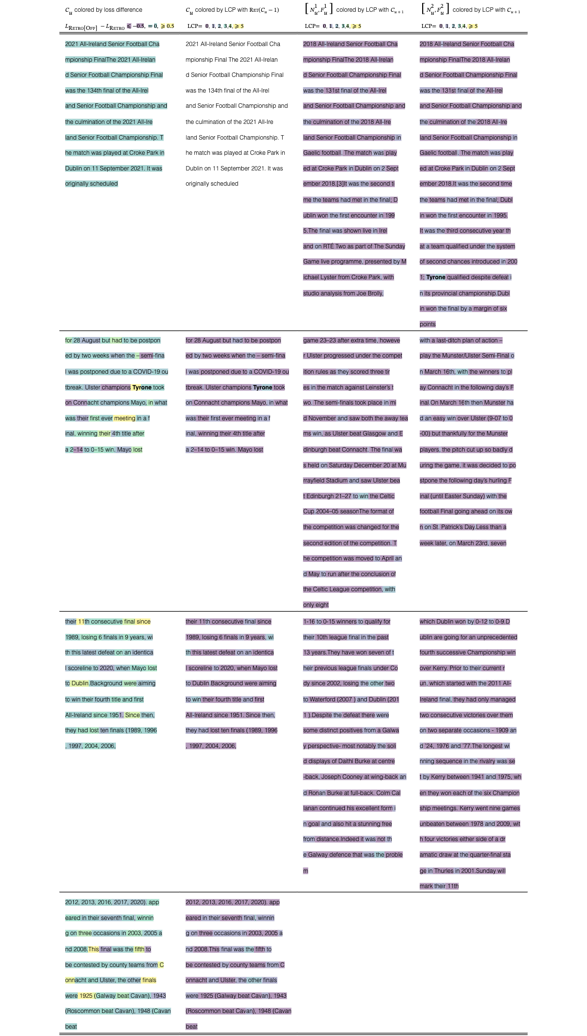
| colored by loss difference | colored by LCP with | colored by LCP with | colored by LCP with |
L_{\textsc{{Retro[Off]} }}-L_{\textsc{Retro}}\hbox{\pagecolor{cm_0!40}\leqslant-0.5},\hbox{\pagecolor{cm_31!40}=0},\hbox{\pagecolor{cm_63!40}\geqslant 0.5} | , , , ,, | , , , ,, | , , , ,, |
| 2020 Summer ParalympicsThe , brand | 2020 Summer Paralympics The , brand | pics Games.* The 2020 Summer Paraly | 2020 Summer ParalympicsThe are an |
| ed as the Tokyo 2020 Paralympic Game | ed as the Tokyo 2020 Paralympic Game | mpics are an upcoming major internat | upcoming major international multi- |
| s, was an international multi-sport | s, was an international multi-sport | ional multi-sport event for athletes | sport event for athletes with disabi |
| parasports event held from 24 August | parasports event held from 24 August | with disabilities governed by the I | lities governed by the International |
| to 5 September 2021 in Tokyo, Japan | to 5 September 2021 in Tokyo, Japan | nternational Paralympic Committee. S | Paralympic Committee. Scheduled as |
| . They were the 16th Summer Paralymp | . They were the 16th Summer Paralymp | cheduled as the 16th Summer Paralymp | the 16th Summer Paralympic Games, th |
| ic Games as organized by the Interna | ic Games as organized by the Interna | ic Games, it is planned to be held i | ey are scheduled to be held in Tokyo |
| tional Paralympic Committee (IPC). | tional Paralympic Committee (IPC). | n Tokyo, Japan from 25 August to 6 S | , Japan between 24 August and 5 Sept |
| eptember 2020.3. 2019 BWF Para-Bad | ember 2021. Originally due to take p | ||
| minton World Championships- The 20 | lace between 25 August and 6 Septemb | ||
| 19 BWF Para-Badminton World Champion | er 2020. On 24 March 2020, the IOC a | ||
| ships was held from 20 to 25 August | nd the Tokyo Organizing Committee of | ||
| 2019 in Basel, Switzerland.- Men’s | ficially announced that the 2020 Sum | ||
| event: Gold Medal: Pramod Bhagat in | mer Olympics and 2020 Summer Paralym | ||
| Singles SL3 Event and Pramod Bhagat | pics would be postponed to 2021, due | ||
| and Manoj | to the COVID-19 pandemic, marking t | ||
| he first time that the Paralympics h | |||
| as been postponed. They will still b | |||
| e publicly marketed as | |||
| Originally scheduled to take place f | Originally scheduled to take place f | once submitted.This process was u | Olympiad, have now been postponed a |
| rom 25 August to 6 September 2020, i | rom 25 August to 6 September 2020, i | ndertaken following the postponement | nd rescheduled for 23 July to 8 Augu |
| n March 2020 both the 2020 Summer Ol | n March 2020 both the 2020 Summer Ol | of the Tokyo 2020 Games due to the | st 2021 in Tokyo, Japan. The Games |
| ympics and Paralympics were postpone | ympics and Paralympics were postpone | COVID-19 pandemic, with both the Oly | were postponed in March 2020 as a re |
| d by one year due to the COVID-19 pa | d by one year due to the COVID-19 pa | mpics and Paralympics pushed back a | sult of the worldwide Covid-19 pande |
| ndemic, with the rescheduled Games s | ndemic, with the rescheduled Games s | year.Now, the Tokyo 2020 Olympics | mic, although they will still keep t |
| till referred to as Tokyo 2020 for m | till referred to as Tokyo 2020 for m | are scheduled for July 23 to August | he name Tokyo 2020 for marketing and |
| arketing and branding purposes. As | arketing and branding purposes. As | 8 while the Paralympics are due to f | branding purposes. This will be th |
| with the Olympics, the Games were la | with the Olympics, the Games were la | ollow from August 24 to September 5. | e first time the Olympic Games have |
| rgely held behind | rgely held behind | The refund process is separate for | been postponed rather than cancelled |
| ticketholders outside of Japan, who | . | ||
| purchased tickets through authorise | |||
| d ticket resellers (ATR).Each ATR | |||
| has its own individual refund proced | |||
| ure.Early figures from the refund | |||
| process for the Tokyo 2020 Olympics | |||
| stated that around 18 per cent | |||
| closed doors with no outside specta | closed doors with no outside specta | has been rescheduled to May 1-4 bec | Olympic Games, when Tokyo became th |
| tors due to a state of emergency in | tors due to a state of emergency in | ause of travel restrictions under th | e first city in Asia to host the Oly |
| the Greater Tokyo Area and other pre | the Greater Tokyo Area and other pre | e current state of emergency in Toky | mpic and Paralympic Games, but unfor |
| fectures. The Games were the second | fectures. The Games were the second | o and other 10 prefectures across Ja | tunately strong winds made it an imp |
| Summer Paralympics hosted by Tokyo s | Summer Paralympics hosted by Tokyo s | pan.The Tokyo 2020 organizing comm | ossible task this time around.Memb |
| ince 1964, and the third Paralympics | ince 1964, and the third Paralympics | ittee announced that the first of 18 | ers of the Tokyo Organising Committe |
| held in Japan overall since the 199 | held in Japan overall since the 199 | test events for the Olympic and Par | e of the Olympic and Paralympic Game |
| 8 Winter Paralympics in Nagano. Th | 8 Winter Paralympics in Nagano. Th | alympic Games will involve wheelchai | s (Tokyo 2020), Tokyo Metropolitan G |
| e Games featured | e Games featured | r rugby, which will be held in Yoyog | overnment officials, Tokyo 2020 Torc |
| i National Stadium from April 3 to 4 | h Relay Official Ambassadors and rep | ||
| .The FINA Diving World Cup will fo | resentatives from Miyagi Prefecture | ||
| llow from April 18 to 23 at the Toky | joined the arrival ceremony.FLAME | ||
| o Aquatics Centre, which will also s | OF RECOVERYThe Olympic flame will | ||
| erve as an Olympic qualifying event. | now be put on display at various loc | ||
| The spread of the COVID-19 pandemi | ations in the Tohoku region, to high | ||
| c has slowed down in Tokyo three wee | light the message of hope in the are | ||
| ks after the Japanese capital entere | as worst affected by the 2011 Great | ||
| d a state of emergency on | East Japan Earthqu | ||
| 539 medal events in 22 sports, with | 539 medal events in 22 sports, with | ||
| badminton and taekwondo both making | badminton and taekwondo both making | ||
| their Paralympic debut to replace f | their Paralympic debut to replace f | ||
| ootball 7-a-side and sailing. China | ootball 7-a-side and sailing. China | ||
| topped the medal table for the fifth | topped the medal table for the fifth | ||
| consecutive Paralympics, with 96 go | consecutive Paralympics, with 96 go | ||
| lds and 207 total medals. Great Brit | lds and 207 total medals. Great Brit | ||
| ain finished second for the ninth t | ain finished second for the ninth t | ||
| ime, | ime, |
View original table
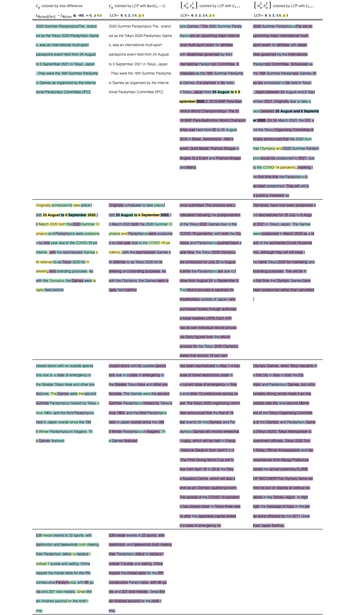
| colored by loss difference | colored by LCP with | colored by LCP with | colored by LCP with |
L_{\textsc{{Retro[Off]} }}-L_{\textsc{Retro}}\hbox{\pagecolor{cm_0!40}\leqslant-0.5},\hbox{\pagecolor{cm_31!40}=0},\hbox{\pagecolor{cm_63!40}\geqslant 0.5} | , , , ,, | , , , ,, | , , , ,, |
| = Daniel Radcliffe =Daniel Jacob R | = Daniel Radcliffe = Daniel Jacob R | Daniel Jacob Radcliffe (born 23 July | Daniel Jacob Radcliffe (born 23 July |
| adcliffe ( born 23 July 1989 ) is an | adcliffe ( born 23 July 1989 ) is an | 1989) is an English actor who rose | 1989) is an English actor who rose |
| English actor who rose to prominenc | English actor who rose to prominenc | to prominence as the title character | to prominence as the title character |
| e as the title character in the Harr | e as the title character in the Harr | in the Harry Potter film series. He | in the Harry Potter film series. He |
| y Potter film series. He made his ac | y Potter film series. He made his ac | made his acting debut at 10 years o | made his acting debut at 10 years o |
| ting debut at 10 years of age in BBC | ting debut at 10 years of age in BBC | f age in BBC One’s 1999 television f | f age in BBC One’s 1999 television m |
| One’s 1999 television film David Co | One’s 1999 television film David Co | ilm David Copperfield, followed by h | ovie David Copperfield, followed by |
| pperfield, followed by his cinematic | pperfield, followed by his cinematic | is cinematic debut in 2001’s The Tai | his film debut in 2001’s The Tailor |
| debut | debut | lor of Panama. At age 11, he was cas | of Panama. At age 11, he was cast as |
| t as Harry Potter in the first Harry | Harry Potter in the first Harry Pot | ||
| Potter film, and starred in the ser | ter film, and starred in the series | ||
| ies for 10 years until the release o | for 10 years until the release of th | ||
| f the eighth and final film in 2011. | e eighth and final film in 2011. Rad | ||
| Radcliffe began to branch out to s | cliffe began to branch out to stage | ||
| tage acting in 2007, starring in the | acting in 2007, starring in the Lond | ||
| London and New York productions of | on and New York productions of Equus | ||
| Equus, and | , and in the | ||
| in 2001’s The Tailor of Panama. At | in 2001’s The Tailor of Panama. At | in 2001’s The Tailor of Panama. At | of Panama. At age 11, he was cast a |
| age 11, he was cast as Harry Potter | age 11, he was cast as Harry Potter | age 11, he was cast as Harry Potter | s Harry Potter in the first Harry Po |
| in the first Harry Potter film, and | in the first Harry Potter film, and | in the first Harry Potter film, and | tter film, and starred in the series |
| starred in the series for 10 years u | starred in the series for 10 years u | starred in the series for 10 years u | for 10 years until the release of t |
| ntil the release of the eighth and f | ntil the release of the eighth and f | ntil the release of the eighth and f | he eighth and final film in 2011.R |
| inal film in 2011.Radcliffe began | inal film in 2011.Radcliffe began | inal film in 2011.Radcliffe began | adcliffe began to branch out to stag |
| to branch out to stage acting in 200 | to branch out to stage acting in 200 | to branch out to stage acting in 200 | e acting in 2007, starring in the Lo |
| 7, starring in the London and New | 7, starring in the London and New | 7, starring in the London and New Yo | ndon and New York productions of Equ |
| rk productions of Equus, and in the | us, and in the 2011 Broadway revival | ||
| 2011 Broadway revival of the musical | of the musical How to Succeed in Bu | ||
| How to Succeed in Business Without | siness Without Really Trying. He sta | ||
| Really Trying. He starred in the 201 | rred in the 2012 horror film The Wom | ||
| 2 horror film The Woman in Black, an | an in Black, and played beat poet Al | ||
| d played beat poet Allen Ginsberg in | len Ginsberg in the 2013 independent | ||
| the 2013 independent film Kill Your | film Kill Your Darlings. He has con | ||
| Darlings.He has contributed to ma | tributed to many charities, includin | ||
| ny charities | g Demelza House Children’s | ||
| York productions of Equus, and in t | York productions of Equus, and in t | York productions of Equus, and in t | in the 2011 Broadway revival of the |
| he 2011 Broadway revival of the musi | he 2011 Broadway revival of the musi | he 2011 Broadway revival of the musi | musical How to Succeed in Business |
| cal How to Succeed in Business Witho | cal How to Succeed in Business Witho | cal How to Succeed in Business Witho | Without Really Trying. He starred in |
| ut Really Trying. He starred in the | ut Really Trying. He starred in the | ut Really Trying. He starred in the | the 2012 horror film The Woman in B |
| 2012 horror film The Woman in Black, | 2012 horror film The Woman in Black, | 2012 horror film The Woman in Black, | lack, and played beat poet Allen Gin |
| and played beat poet Allen Ginsberg | and played beat poet Allen Ginsberg | and played beat poet Allen Ginsberg | sberg in the 2013 independent film K |
| in the 2013 independent film Kill Y | in the 2013 independent film Kill Y | in the 2013 independent film Kill Y | ill Your Darlings. He has contribute |
| our <unk>.He has contributed to ma | our <unk>.He has contributed to ma | our Darlings.He has contributed to | d to many charities, including Demel |
| ny charities, | ny charities, | many charities, including Demelza H | za House Children’s Hospice and The |
| ouse Children’s Hospice and The Trev | Trevor Project. He also made public | ||
| or Project. He also made public serv | service announcements for the latter | ||
| ice announcements for the latter. In | . In 2011, he was awarded the Trevor | ||
| 2011, he was awarded the Trevor Pro | Project’s "Hero Award." | ||
| ject’s "Hero Award."Sources disagr | |||
| ee about Radcliffe’s personal wealth | |||
| ; he was reported to have earned £1 | |||
| million for the first Harry Potter | |||
| including <unk> Hospice Care for Ch | including <unk> Hospice Care for Ch | ||
| ildren, and The Trevor Project for s | ildren, and The Trevor Project for s | ||
| uicide prevention among LGBTQ youth, | uicide prevention among LGBTQ youth, | ||
| which gave him its Hero Award in 20 | which gave him its Hero Award in 20 | ||
| 11.= = Early life = =Radcliffe w | 11.= = Early life = =Radcliffe w | ||
| as born in West London, England. He | as born in West London, England. He | ||
| is the only child of Alan George Rad | is the only child of Alan George Rad | ||
| cliffe, a literary agent, and | cliffe, a literary agent, and |
View original table
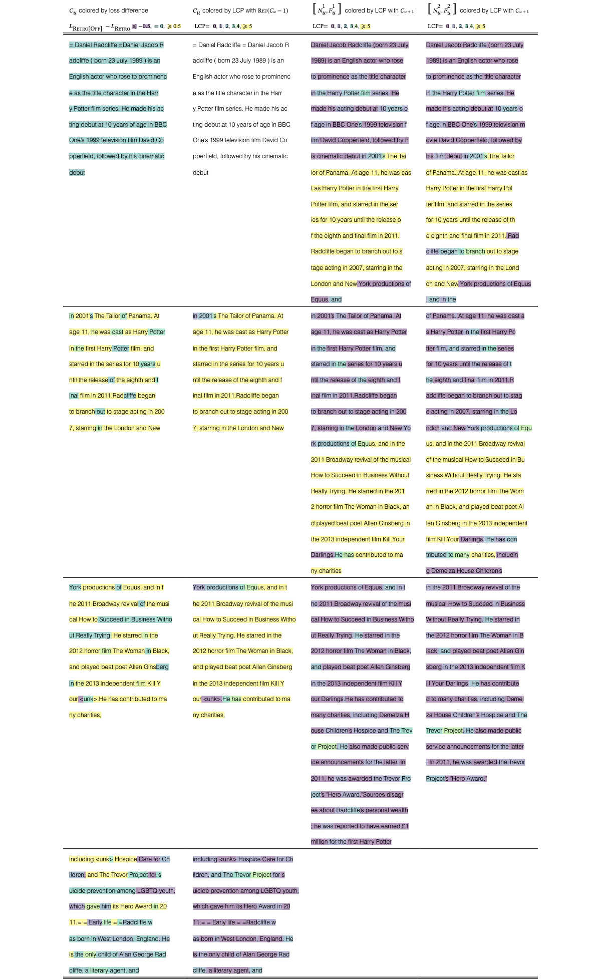
| Prompt and sample of Retro[Off] | Prompt and sample of Retro[On] | colored by LCP with | colored by LCP with |
| colored by LCP with | |||
| , , , ,, | , , , ,, | , , , ,, | |
| Article premier - Les hommes | Article premier - Les hommes | de l’homme et du citoyen.Ar | Les hommes naissent et demeur |
| naissent et demeurent libres e | naissent et demeurent libres e | ticle 1erLes hommes naissent | ent libres et égaux en droits. |
| t égaux en droits. Les distinc | t égaux en droits. Les distinc | et demeurent libres et égaux | Les distinctions sociales ne |
| tions sociales ne peuvent être | tions sociales ne peuvent être | en droits. Les distinctions so | peuvent être fondées que sur l |
| fondées que sur l’utilité com | fondées que sur l’utilité com | ciales ne peuvent être fondées | ’utilité commune.Art. 2. - |
| mune. Article 2. - Le but de | mune. Article 2. - Le but de | que sur l’utilité commune.A | Le but de toute association po |
| toute association politique e | toute association politique e | rticle 2Le but de toute asso | litique est la conservation de |
| st la conservation des droits | st la conservation des droits | ciation politique est la conse | s droits naturels et imprescri |
| naturels et | naturels et | rvation des droits naturels et | ptibles de l’Homme. Ces droits |
| imprescriptibles de l’homme. | sont la liberté, la propriété | ||
| Ces droits sont la liberté, la | , la sûreté, et la résistance | ||
| propriété, la sûreté, et la r | à l’oppression.Art. 3. -Le | ||
| ésistance à l’oppression.Art | principe de toute Souverainet | ||
| icle 3Le principe de toute s | é réside essentiellement dans | ||
| ouveraineté réside essentielle | la Nation. Nul corps, nul indi | ||
| ment dans la nation. Nul corps | vidu ne peut exercer d’autorit | ||
| , nul individu ne peut exercer | é qui n’en émane expressément. | ||
| d’autorité qui n’en | Art | ||
| imprescriptibles de l’homme, | imprescriptibles de l’homme. | criptibles del’homme. Ces dro | et imprescriptibles de l’homm |
| et par conséquent la garantie | Ces droits sont la liberté, la | its sont la liberté, la propri | e. Ces droits sont la liberté, |
| à chacun des droits suivants | propriété, la sûreté et la ré | été, la sûretéet la résistanc | la propriété, la sûreté et la |
| : Article 3. - La propriété | sistance à l’oppression.Arti | e à l’oppression.Article 3 - | résistance à l’oppression.A |
| est un droit inviolable et sa | cle 3.- Le principe de toute | Le principe de toute souverai | rticle 3 - Le principe de tout |
| cré. Toute personne a le droit | souveraineté réside essentiel | neté résideessentiellement da | e souveraineté réside essentie |
| de procéder à sa propre cons | lement dans la nation. Nul cor | ns la Nation. Nul corps, nul i | llement dans la Nation. Nul co |
| ervation. Article 4. - Le | ps, nul individu ne peut exerc | ndividu nepeut exercer d’auto | rps, nul individu ne peut exer |
| er d’autorité qui n | rité qui n’en émane expresséme | cer d’autorité qui n’en émane | |
| nt.Article 4 - La liberté co | expressément.Article 4 - La | ||
| nsiste à pouvoir faire tout ce | liberté consiste à pouvoir fai | ||
| quine nuit pas à autrui : ai | re tout ce qui ne nuit pas à a | ||
| nsi, l’exercice des droits nat | utrui : ainsi, l’exercice des | ||
| urelsde chaque homme n’a de b | droits naturels de chaque homm | ||
| ornes que celles qui assurent | e n’a de bornes que celles qui | ||
| auxautres membres de la socié | assurent aux autres membres d | ||
| té la jouissance de | e la société la jouissance de | ||
| ces mêmes droits. Ces bornes | |||
| but de toute association est | ’en émane expressément.Artic | mane expressément.Article 4 | mane expressément.Article 4 |
| la défense des droits de l’hom | le 4.- La liberté consiste à | - La liberté consiste à pouvoi | - La liberté consiste à pouvoi |
| me et du citoyen. Tout citoye | pouvoir faire tout ce qui ne | r faire tout ce qui ne nuit pa | r faire tout ce qui ne nuit pa |
| n a le droit de participer à l | nuit pas à autrui : ainsi, l’e | s à autrui : ainsi, l’exercice | s à autrui : ainsi, l’exercice |
| a direction des affaires publi | xercice des droits naturels de | des droits naturels de chaque | des droits naturels de chaque |
| ques. Article 5. - L’impuni | chaque homme n’a de bornes qu | homme n’a de bornes que celle | homme n’a de bornes que celle |
| té n’a jamais été et ne sera j | e celles qui assurent aux autr | s qui assurent aux autres memb | s qui assurent aux autres memb |
| amais une fin en elle-même. L’ | es membres de la société la jo | res de la société la jouissanc | res de la société la jouissanc |
| imp | uissance de ces mêmes | e de ces mêmes droits. Ces bor | e de ces mêmes droits. Ces bor |
| nes ne peuvent être déterminée | nes ne peuvent être déterminée | ||
| s que par la loi.Article 5 - | s que par la loi.Article 5 - | ||
| La loi n’a le droit de défend | La loi n’a le droit de défend | ||
| re que les actions nuisibles à | re que les actions nuisibles à | ||
| la société. Tout ce qui n’est | la société. Tout ce qui n’est | ||
| pas défendu par la loi ne peu | pas défendu par la loi ne peu | ||
| t être empêché, et nul ne peut | t être empêché, et nul ne peut | ||
| être contraint à faire ce qu’ | être contraint à faire ce qu’ | ||
| elle n | elle n | ||
| unité, comme le despotisme, s | droits. Ces bornes ne peuvent | ||
| ’est toujours révélée être un | être déterminées que par la l | ||
| instrument d’oppression. La ty | oi.Article 5.- La loi n’a | ||
| rannie qui s’est élue juge su | le droit de défendre que les a | ||
| prême de la conscience des aut | ctions nuisibles à la société. | ||
| res ne peut être jugée. La jus | Tout ce qui n’est pas défendu | ||
| tice se trouve dans la consci | par la loi ne peut être empêc | ||
| ence de chaque citoyen, | hé, et nul ne peut être |
View original table
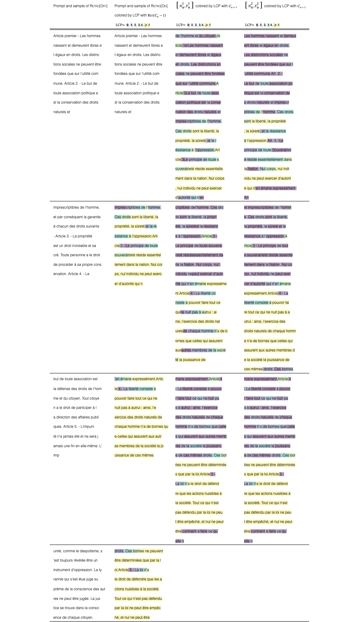
| Prompt and sample of Retro[Off] | Prompt and sample of Retro[On] | colored by LCP with | colored by LCP with |
|---|---|---|---|
| colored by LCP with | |||
| , , , ,, | , , , ,, | , , , ,, | |
| Pi = 3. 1415926535 8979323846 | Pi = 3. 1415926535 8979323846 | “1415926535 8979323846 26433 | 46 2643383279 5028841971 69399 |
| 2643383279 5028841971 69399375 | 2643383279 5028841971 69399375 | 83279 5028841971 693993751058 | 37510 5820974944 592307816406 |
| 10 5820974944 5923078164 06286 | 10 5820974944 5923078164 06286 | 20974944 5923078164 0628620899 | 28620899 8628034825 3421170679 |
| 20899 8628034825 3421170679 | 20899 8628034825 3421170679 | 8628034825 34211706798214808 | 8214808651 3282306647 0938446 |
| 651 3282306647 0938446095 5058 | 095 50582231725359408128 4811 | ||
| 223172 53594081284811174502 8 | 174502 8410270193 8521105559 6 | ||
| 410270193 8521105559 644622948 | 446229489 5493038196 442881097 | ||
| 9 54930381964428810975 665933 | 56659334461 2847564823 378678 | ||
| 4461 2847564823 3786783 | 3165 2712019091 4564856692 346 | ||
| 0 | |||
| 8294049602 8988496069 9858349 | 8214808651 3282306647 0938446 | 651 3282306647 0938446095 5058 | 47 0938446095 5058223172 53594 |
| 065 9873246379 9644789435 8628 | 095 5058223172 53594081284811 | 223172 5359408128 4811174502 | 081284811174502 8410270193 85 |
| 730709 6540159079 5944069810 5 | 174502 8410270193 8521105559 6 | 8410270193 8521105559 64462294 | 21105559 6446229489 5493038196 |
| 992965913 7095378412 69378359 | 446229489 5493038196442881097 | 89 54930381964428810975 66593 | 4428810975 6659334461 2847564 |
| 5 6659334461 284 | 34461 2847564823 3786783165 27 | 823 3786783165 27120190914564 | |
| 12019091 4564856692 346034861 | 856692 3460348610 4543266482 1 | ||
| 0 4543266482 1339360726 024914 | 339360726 0249141273724587006 | ||
| 12737245870066 0631558817 488 | 6 0631558817 4881520920 962829 | ||
| 1520920 9628292540 91715364 | 2540 91715364367892590360 | ||
| 10 6940372045 7088679512 85612 | 7564823 3786783165 2712019091 | 23 3786783165 2712019091 4564 | 165 27120190914564856692 3460 |
| 30857 9046461290 9276642155 56 | 4564856692 3460348610 45432664 | 856692 3460348610 4543266482 1 | 348610 4543266482 1339360726 0 |
| 54603269 5656128798 6366475705 | 82 1339360726 024914127372458 | 339360726 0249141273724587006 | 2491412737245870066 063155881 |
| 6294954741 5886335339 57657 | 70066 0631558817 4881520920 96 | 6 0631558817 4881520920 962829 | 7 4881520920 9628292540 917153 |
| 28292540 91715 | 2540 9171536436 7892590360 01 | 64367892590360 0113305305 488 | |
| 13305305 4882046652 1384146951 | 2046652 1384146951 9415116094 | ||
| 94151160943305727036 5759591 | 3305727036 5759591953 09218611 | ||
| 953 0921861173 8193261179 3105 | 73 8193261179 310511854807446 | ||
| 118548 0744623799 627495 | 23799 6274956735 1885752724 89 | ||
| 1227 | |||
| 76345 5770886953 7988876910 79 | 364367892590360 0113305305 48 | ||
| 66169745 6493974637 6345801550 | 82046652 1384146951 9415116094 | ||
| 6663542854 6333764630 6356284 | 3305727036 5759591953 0921861 | ||
| 271 7885339804 5672434 | 173 8193261179 31051185480744 | ||
| 623799 6274 |
View original table