Transformers are SSMs: Generalized Models and Efficient Algorithms Through Structured State Space Duality

Tri Dao, Albert Gu

arXiv:2405.21060v1 · This workspace stays on this version. Check arXiv for newer versions

Affiliations and author notes

tri@tridao.me, agu@cs.cmu.edu
Department of Computer Science, Princeton University
Machine Learning Department, Carnegie Mellon University
Alphabetical by last name.

Some source details need review 1 to check

Original formulas, table values and figures are preserved. Comparison can miss differences; use the original PDF to check details.

Reading view checked: 1049 math expressions, 0 rendering failures; 20 of 20 images available.

Compared 319 of 585 source passages against 32 of 52 PDF pages.

The HTML source contains failed formatting commands; these were omitted from the reading view. The original sources are retained. (1)

This long paper was only partially compared; the original sources remain available.

20 of 20 figure, table and graphic images captured. Open original PDF

Abstract

While Transformers have been the main architecture behind deep learning’s success in language modeling, state-space models (SSMs) such as Mamba have recently been shown to match or outperform Transformers at small to medium scale. We show that these families of models are actually quite closely related, and develop a rich framework of theoretical connections between SSMs and variants of attention, connected through various decompositions of a well-studied class of structured semiseparable matrices. Our state space duality (SSD) framework allows us to design a new architecture (Mamba-2) whose core layer is an a refinement of Mamba’s selective SSM that is 2-8 $\times$ faster, while continuing to be competitive with Transformers on language modeling.

Transformers, in particular decoder-only models (e.g. GPT (Brown et al., 2020), Llama (Touvron et al., 2023)) which process input sequences in a causal fashion, are one of the main drivers of modern deep learning’s success. Numerous approaches attempt to approximate the core attention layer to address its efficiency issues (Tay et al., 2022), such as scaling quadratically in sequence length during training and requiring a cache of size linear in sequence length during autoregressive generation. In parallel, a class of alternative sequence models, structured state-space models (SSMs), have emerged with linear scaling in sequence length during training and constant state size during generation. They show strong performance on long-range tasks (e.g. S4 (Gu et al., 2022)) and recently matched or beat Transformers on language modeling (e.g. Mamba (Gu & Dao, 2023)) at small to moderate scale. However, the development of SSMs have appeared disjoint from the community’s collective effort to improve Transformers, such as understanding them theoretically as well as optimizing them on modern hardware. As a result, it is more difficult to understand and experiment with SSMs compared to Transformers, and it remains challenging to train SSMs as efficiently as Transformers from both an algorithmic and systems perspective.

Our main goal is to develop a rich body of theoretical connections between structured SSMs and variants of attention. This will allow us to transfer algorithmic and systems optimizations originally developed for Transformers to SSMs, towards the goal of building foundation models that perform better than Transformers while scaling more efficiently in sequence length. A milestone contribution in this direction was the Linear Attention (LA) framework (Katharopoulos et al., 2020), which derived a connection between autoregressive attention and linear RNNs by showing the equivalence between ‘‘dual forms’’ of quadratic kernelized attention and a particular linear recurrence. This duality allows new capabilities such as the ability to have both efficient parallelizable training and efficient autoregressive inference. In the same spirit, this paper provides multiple viewpoints connecting linear-complexity SSMs with quadratic-complexity forms to combine the strengths of SSMs and attention. $^{1}$

Figure 1: (**Structured State-Space Duality**.) This paper fleshes out the relationship between state space models and attention through the bridge of structured matrices.

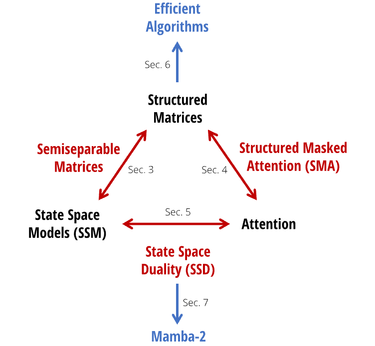
Our framework connecting structured SSMs and variants of attention, which we call structured state space duality (SSD), is made through the abstractions of structured matrices: matrices with subquadratic parameters and multiplication complexity. We develop two broad frameworks for representing sequence models, one as matrix transformations and one as tensor contractions, which each reveal different perspectives of the duality. Our technical contributions include:

•
We show an equivalence between state space models and a well-studied family of structured matrices called semiseparable matrices (Section 3). This connection is at the heart our framework, revealing new properties and algorithms for SSMs. A central message of this paper is that different methods of computing state space models can be reframed as various matrix multiplication algorithms on structured matrices.
•
We significantly improve the theory of linear attention (Katharopoulos et al., 2020). We first provide an incisive proof of its recurrent form through the language of tensor contractions, and then generalize it to a new family of structured masked attention (SMA) (Section 4).
•
We connect SSMs and SMA, showing that they have a large intersection that are duals of each other, possessing both SSM-like linear and attention-like quadratic forms (Section 5). We also prove that any kernel attention method possessing a fast recurrent form must be an SSM.

Beyond its intrinsic theoretical value, our framework opens up a broad set of directions for understanding and improving sequence models.

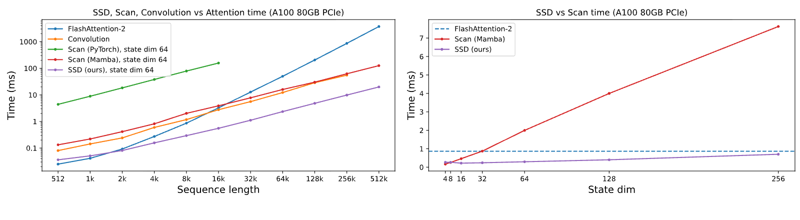
First and most importantly, our framework exposes new efficient and easily-implementable algorithms for computing SSMs (Section 6). We introduce a new SSD algorithm, based on block decompositions of semiseparable matrices, that takes advantage of both the linear SSM recurrence and quadratic dual form, obtaining optimal tradeoffs on all main efficiency axes (e.g. training and inference compute, memory usage, and ability to leverage matrix multiplication units on modern hardware). A dedicated implementation of SSD is $2-8\times$ faster than the optimized selective scan implementation of Mamba, while simultaneously allowing for much larger recurrent state sizes ( $8\times$ the size of Mamba or even higher, with minimal slowdown). SSD is highly competitive with optimized implementations of softmax attention (FlashAttention-2 (Dao, 2024)), crossing over at sequence length 2K and 6 $\times$ faster at sequence length 16K.

One major obstacle to adopting new architectures such as SSMs is the ecosystem tailored to Transformers, such as hardware-efficient optimization and parallelism techniques for large-scale training. Our framework allows using established conventions and techniques for attention to build a vocabulary of architecture design choices for SSMs, and further improve them (Section 7). For example, we introduce the analog of heads from multi-head attention (MHA) to SSMs. We show that the Mamba architecture is a multi-input SSM (MIS) that turns out to be analogous to multi-value attention (MVA), and compare other variants of Mamba with different head structures.

We also use these ideas to make slight modifications to the Mamba block, which allows tensor parallelism to be implemented (e.g. in the style of Megatron (Shoeybi et al., 2019)). The main ideas include introducing grouped-value attention (GVA) head structure, and moving all data-dependent projections to occur in parallel at the beginning of the block.

The combination of the modified parallel Mamba block, together with using SSD as the inner SSM layer, results in the Mamba-2 architecture. We investigate Chinchilla scaling laws for Mamba-2 in the same setting as Mamba, finding that it Pareto dominates Mamba and Transformer++ in both perplexity and wall-clock time. We additionally train a family of Mamba-2 models at varying sizes on the Pile, showing that it matches or outperforms Mamba and open source Transformers on standard downstream evaluations. For example, Mamba-2 with 2.7B parameters trained on 300B tokens on the Pile outperforms Mamba-2.8B, Pythia-2.8B and even Pythia-6.9B trained on the same dataset.

The SSD framework connects SSMs and Transformers, allowing us to leverage a rich body of work on systems optimizations developed for Transformers (Section 8).

•
For example, Tensor Parallelism (TP) is an important model parallelism technique to train large Transformer models by splitting each layer across GPUs on the same node. We design Mamba-2 to be TP-friendly, reducing the number of synchronization point per block by half.
•
For very long sequences whose activations do not fit on one device, sequence parallelism has been developed for the attention blocks. We describe how to train SSMs in general and Mamba-2 in particular with sequence parallelism, by passing the recurrent states between devices.
•
For finetuning with examples of different lengths, for best efficiency, Transformer requires sophisticated techniques to remove padding tokens and perform attention on variable length sequences. We show how Mamba-2 can be trained with variable sequence lengths efficiently, requiring no padding tokens.

Section 9 empirically validates Mamba-2 on language modeling, training efficiency, and a difficult multi-query associative recall task (Arora et al., 2024a). Finally, in Section 10, we provide an extended related work and discuss potential research directions opened up by our framework.

Model code and pre-trained checkpoints are open-sourced at https://github.com/state-spaces/mamba.

Structured state space sequence models (S4) are a recent class of sequence models for deep learning that are broadly related to RNNs, CNNs, and classical state space models. They are inspired by a particular continuous system (1) that maps a 1-dimensional sequence $x\in\mathbb{R}^{\mathtt{T}}\mapsto y\in\mathbb{R}^{\mathtt{T}}$ through an implicit latent state $h\in\mathbb{R}^{\mathtt{(T,N)}}$ .

A general discrete form of structured SSMs takes the form of equation (1).

\begin{aligned}\displaystyle h_{t} & \displaystyle=Ah_{t-1}+Bx_{t} \\ \displaystyle y_{t} & \displaystyle=C^{\top}h_{t}\end{aligned}

\begin{aligned}\displaystyle h_{t} & \displaystyle=A_{t}h_{t-1}+B_{t}x_{t} \\ \displaystyle y_{t} & \displaystyle=C_{t}^{\top}h_{t}\end{aligned}

where $A\in\mathbb{R}^{\mathtt{(N,N)}},B\in\mathbb{R}^{\mathtt{(N,1)}},C\in\mathbb{R}^{\mathtt{(N,1)}}$ . Structured SSMs are so named because the $A$ matrix controlling the temporal dynamics must be structured in order to compute this sequence-to-sequence transformation efficiently enough to be used in deep neural networks. The original structures introduced were diagonal plus low-rank (DPLR) (Gu et al., 2022) and diagonal (Gupta et al., 2022; Gu et al., 2022a; Smith et al., 2023), which remains the most popular structure.

In this work, we use the term state space model (SSM) to refer to structured SSMs. There are many flavors of such SSMs, with deep ties to several major paradigms of neural sequence models such as continuous-time, recurrent, and convolutional models (Gu et al., 2021). We provide a brief overview below, and refer to prior work for more context and details (Gu, 2023; Gu & Dao, 2023).

The original structured SSMs originated as continuous-time maps on functions $x(t)\in\mathbb{R}\mapsto y(t)\in\mathbb{R}$ , rather than operating directly on sequences. In the continuous-time perspective, in equation (1a) the matrices $(A,B)$ are not directly learned but generated from underlying parameters $(\mathring{A},\mathring{B})$ , along with a parameterized step size $\Delta$ . The “continuous parameters” $(\Delta,\mathring{A},\mathring{B})$ are converted to “discrete parameters” $(A,B)$ through fixed formulas $A=f_{A}(\Delta,\mathring{A})$ and $B=f_{B}(\Delta,\mathring{B})$ , where the pair $(f_{A},f_{B})$ is called a discretization rule.

Remark 1.

While our main models adopt the same parameterization and discretization step as prior work (see Gu & Dao (2023) for details), for simplifying exposition and notation we omit it in the rest of this paper. We note that prior work on structured SSMs referred to the continuous parameters $(\mathring{A},\mathring{B})$ and discrete parameters $(A,B)$ as $(A,B)$ and $(\bar{A},\bar{B})$ instead; we have changed notation to simplify the presentation and focus directly on the discrete parameters, which govern the main SSM recurrence.

Equations (1) and (2) take the form of a recurrence which is linear in its input $x$ . Structured SSMs can therefore be viewed as types of recurrent neural networks (RNNs), where the linearity endows them with additional properties and allows them to avoid the sequential computation of traditional RNNs. Conversely, despite this simplification, SSMs are still fully expressive as sequence transformations (in the sense of universal approximation) (Kaul, 2020; Orvieto et al., 2023; Wang & Xue, 2023).

When the SSM’s dynamics are constant through time as in equation (1), the model is called linear time-invariant (LTI). In this case, they are equivalent to convolutions. Thus, SSMs can also be viewed as types of CNNs, but where (i) the convolution kernels are implicitly parameterized through the SSM parameters $(A,B,C)$ and (ii) the convolution kernels are generally global instead of local. Conversely, through classical signal processing theory all sufficiently well-behaved convolutions can be represented as SSMs.

Commonly, previous LTI SSMs would use the convolutional mode for efficient parallelizable training (where the whole input sequence is seen ahead of time), and switched into recurrent mode (1) for efficient autoregressive inference (where the inputs are seen one step at a time).

The form (2) where the parameters $(A,B,C)$ can also vary in time was introduced in Mamba as the selective SSM. Compared to the standard LTI formulation (1), this model can selectively choose to focus on or ignore inputs at every timestep. It was shown to perform much better than LTI SSMs on information-dense data such as language, especially as its state size $\mathtt{N}$ increases allowing for more information capacity. However, it can only be computed in recurrent instead of convolutional mode, and requires a careful hardware-aware implementation to be efficient. Even so, it is still less efficient than hardware-friendly models such as CNNs and Transformers because it does not leverage matrix multiplication units, which modern accelerators such as GPUs and TPUs are specialized for.

While time-invariant SSMs are closely related to continuous, recurrent, and convolutional sequence models, they are not directly related to attention. In this paper, we show a deeper relationship between selective SSMs and attention, and use it to significantly improve the training speed of SSMs while simultaneously allowing for much larger state sizes $\mathtt{N}$ .

Definition 2.1.

We use the term sequence transformation to refer to a parameterized map on sequences $Y=f_{\theta}(X)$ where $X,Y\in\mathbb{R}^{\mathtt{(T,P)}}$ and $\theta$ is an arbitrary collection of parameters. $\mathtt{T}$ represents the sequence or time axis; subscripts index into the first dimension, e.g. $X_{t},Y_{t}\in\mathbb{R}^{\mathtt{P}}$ .

Sequence transformations (e.g. SSMs, or self-attention) are the cornerstone of deep sequence models, where they are incorporated into neural network architectures (e.g. Transformers). The SSM in (1) or (2) is a sequence transformation with $\mathtt{P}=1$ ; it can be generalized to $\mathtt{P}>1$ by simply broadcasting across this dimension (in other words, viewing the input as $\mathtt{P}$ independent sequences and applying the SSM to each). One can think of $\mathtt{P}$ as a head dimension, which we will elaborate on in Section 7.

Definition 2.2.

We define the SSM operator $\mathsf{SSM}(A,B,C)=\mathsf{SSM}(A_{0:T},B_{0:T},C_{0:T})$ as the sequence transformation $X\in\mathbb{R}^{\mathtt{(T,P)}}\mapsto Y\in\mathbb{R}^{\mathtt{(T,P)}}$ defined by equation (2).

In SSMs, the $\mathtt{N}$ dimension is a free parameter called the state size or state dimension. We also call it the state expansion factor, because it expands the size of the input/output by a factor of $N$ , with implications for the computational efficiency of these models.

Finally, we remark that many types of sequence transformations, such as attention, can be represented as a single matrix multiplication across the sequence dimension.

Definition 2.3.

We call a sequence transformation $Y=f_{\theta}(X)$ a matrix transformation if it can be written in the form $Y=M_{\theta}X$ where $M$ is a matrix depending on the parameters $\theta$ . We identify the sequence transformation with the matrix $M$ , and often drop the dependence on $\theta$ when clear from context.

Attention broadly refers to a type of computation that assigns scores to every pair of positions in a sequence, allowing each element to “attend” to the rest. By far the most common and important variant of attention is softmax self-attention, which can be defined as

\displaystyle Y=\operatorname*{softmax}(QK^{\top})\cdot V

for $Q,K,V\in\mathbb{R}^{\mathtt{(T,P)}}$ . The mechanism of pairwise comparisons (induced by materializing $QK^{\top}$ ) leads to the characteristic quadratic training cost of attention.

Many variants of attention have been proposed, but all share the underlying core of these attention scores, with various approximations (Tay et al., 2022). The most important variant for this work is linear attention (Katharopoulos et al., 2020). Roughly speaking, this family of methods drops the softmax by folding it into a kernel feature map, and uses associativity of matrix multiplication to rewrite $(QK^{\top})\cdot V=Q\cdot(K^{\top}V)$ . Moreover, in the important case of causal (autoregressive) attention, they show that when the causal mask is incorporated into the left-hand side as $(L\circ QK^{\top})\cdot V$ , where $L$ is the lower-triangular 1’s matrix, then the right-hand side can be expanded as a recurrence. Several recent and concurrent works such as RetNet (Sun et al., 2023) and GateLoop (Katsch, 2023) strengthen this to more general forms of $L$ (Section 10). In this work, our formulation of structured masked attention will strongly generalize these ideas.

General matrices $M\in\mathbb{R}^{\mathtt{(T,T)}}$ require $\mathtt{T}^{2}$ parameters to represent and $O(\mathtt{T}^{2})$ time to perform basic operations such as matrix-vector multiplication. Structured matrices are those that

(i)
can be represented in subquadratic (ideally linear) parameters through a compressed representation, and
(ii)
have fast algorithms (most importantly matrix multiplication) by operating directly on this compressed representation.

Perhaps the most canonical families of structured matrices are sparse and low-rank matrices. However, there exist many other families, such as Toeplitz, Cauchy, Vandermonde, and butterfly matrices, which have all been used in machine learning for efficient models (Thomas et al., 2018; Dao et al., 2019; Gu et al., 2022a; Fu et al., 2024). Structured matrices are a powerful abstraction for efficient representations and algorithms. In this work, we will show that SSMs are equivalent to another class of structured matrices that have not previously been used in deep learning, and use this connection to derive efficient methods and algorithms.

While this paper develops a much richer framework of connections between SSMs, attention, and structured matrices, we provide a brief summary of the main method, which is actually quite self-contained and simple algorithmically.

The state space dual (SSD) layer can be defined as a special case of the selective SSM (2). The standard computation of an SSM as a recurrence (or parallel scan) can be applied, which has linear complexity in sequence length. Compared to the version used in Mamba, SSD has two minor differences:

•
The structure on $A$ is further simplified from diagonal to scalar times identity structure. Each $A_{t}$ can also be identified with just a scalar in this case.
•
We use a larger head dimension $\mathtt{P}$ , compared to $\mathtt{P}=1$ used in Mamba. Typically $\mathtt{P}=\{64,128\}$ is chosen which is similar to conventions for modern Transformers.

Compared to the original selective SSM, these changes can be viewed as slightly decreasing the expressive power in return for significant training efficiency improvements. In particular, our new algorithms will allow the use of matrix multiplication units on modern accelerators.

The dual form of SSD is a quadratic computation closely related to attention, defined as

\displaystyle(L\circ QK^{\top})\cdot V\qquad L_{ij}=\begin{cases}a_{i}\times\dots\times a_{j+1}&i\geq j\\ 0&i<j\end{cases}

where $a_{i}$ are input-dependent scalars bounded in $[0,1]$ .

Compared to standard softmax attention, there are two main differences

•
The softmax is dropped.
•
The attention matrix is multiplied elementwise-wise by an additional mask matrix $L$ .

Both of these changes can be viewed as addressing problems in vanilla attention. For example, the softmax has been recently observed to cause problems in attention scores, such as the “attention sink” phenomenon (Xiao et al., 2024; Darcet et al., 2024). More importantly, the mask matrix $L$ can be viewed as replacing the heuristic positional embeddings of Transformers with a different data-dependent positional mask that controls how much information is transfered across time.

More broadly, this form is an instance of our structured masked attention generalization of linear attention, defined in Section 4.

The various forms of SSD are connected through a unified matrix representation, by showing that SSMs have a matrix transformation form $Y=MX$ for a matrix $M_{\theta}\in\mathbb{R}^{\mathtt{(T,T)}}$ that depends on $\theta=(A,B,C)$ . In particular, the dual form of SSD is equivalent to naive (quadratic-time) multiplication by the matrix $M$ , and the recurrent form is a particular efficient (linear-time) algorithm that leverages the structure in $M$ .

Going beyond these, any algorithm for multiplication by $M$ can be applied. Our proposed hardware-efficient SSD algorithm (Section 6) is a new structured matrix multiplication method that involves block decompositions of $M$ , which obtains better efficiency tradeoffs than either the pure linear or quadratic forms. It is relatively simple and easy-to-implement compared to general selective SSMs (Gu & Dao, 2023); Section 6.2 provides a complete implementation in a few lines of code.

Figure 1 provides a simple roadmap of the relationships between the concepts presented in this paper.

Throughout this paper, we prefer using precise notation that can be mapped to code.

We generally use lower case to denote vectors (i.e. tensors with a single axis) and upper case to denote matrices (i.e. tensors with more than one axes). We do not bold matrices in this work. Sometimes, if a matrix is tied or repeated along one axis (and hence can also be viewed as a vector), we may use either upper or lower case for it. $^{2}$ $\cdot$ denotes scalar or matrix multiplication while $\circ$ denotes Hadamard (elementwise) multiplication.

We use Python-style indexing, e.g. $i:j$ refers to the range $(i,i+1,\dots,j-1)$ when $i<j$ and $(i,i-1,\dots,j+1)$ when $i>j$ . For example, for any symbol $v$ we let $v_{j:i}$ for $j\geq i$ denote the sequence $(v_{j},\dots,v_{i+1})$ . $[i]$ is equivalent to $0:i=(0,\dots,i-1)$ . For shorthand, we also let $v_{j:i}^{\times}$ denote the product $v_{j}\times\dots\times v_{i+1}$ . $^{3}$

To distinguish from matrices and tensors, we often use capital letters in typewriter fonts (e.g. $\mathtt{D},\mathtt{N},\mathtt{T})$ to denote dimensions and tensor shapes. Instead of the traditional notation $M\in\mathbb{R}^{T\times T}$ we frequently use $M\in\mathbb{R}^{\mathtt{(T,T)}}$ to reflect tensor shapes in code.

We will heavily rely on tensor contraction or einsum notation both for clarity and as a central tool in stating and proving our results. We assume the reader to be familiar with this notation, which is commonly used in modern tensor libraries such as numpy. For example, we can use $\mathsf{contract}(\mathtt{MN,NK\to MK})$ to denote the matrix-matrix multiplication operator, and in our notation $\mathsf{contract}(\mathtt{MN,NK\to MK})(X,Y)$ (which is equivalent to $X\cdot Y$ ) can be translated to code as $\mathtt{numpy.einsum(^{\prime}mn,nk\to mk^{\prime},X,Y)}$ .

A large glossary of notation is included in Appendix A.

This section explores different perspectives of the state space model as a sequence transformation, and outlines properties and algorithms of such maps. The main results of this section are about the equivalence between state space models and a family of structured matrices called semiseparable matrices, which imply new efficiency results (Theorems 3.5 and 3.7).

Recall that our definition of an SSM is defined as a parameterized map defined through (2). Our theoretical framework starts by simply writing this transformation as a matrix multiplication mapping the vectors $x\in\mathbb{R}^{\mathtt{T}}\mapsto y\in\mathbb{R}^{\mathtt{T}}$ .

By definition, $h_{0}=B_{0}x_{0}$ . By induction,

\begin{aligned}\displaystyle h_{t} & \displaystyle=A_{t}\dots A_{1}B_{0}x_{0}+A_{t}\dots A_{2}B_{1}x_{1}+\dots+A_{t}A_{t-1}B_{t-2}x_{t-2}+A_{t}B_{t-1}x_{t-1}+B_{t}x_{t}\end{aligned}

\begin{aligned} & \displaystyle=\sum_{s=0}^{t}A_{t:s}^{\times}B_{s}x_{s}.\end{aligned}

Multiplying by $C_{t}$ to produce $y_{t}$ and vectorizing the equation over $t\in[\mathtt{T}]$ , we derive the matrix transformation form of SSMs.

\begin{aligned}\displaystyle y_{t} & \displaystyle=\sum_{s=0}^{t}C_{t}^{\top}A_{t:s}^{\times}B_{s}x_{s} \\ \displaystyle y & \displaystyle=\mathsf{SSM}(A,B,C)(x)=Mx \\ \displaystyle M_{ji} & \displaystyle\coloneqq C_{j}^{\top}A_{j}\cdots A_{i+1}B_{i}\end{aligned}

$M$ in equation (3) is a particular representation of a class of matrices known as semiseparable matrices. Semiseparable matrices are a fundamental matrix structure. We first define these matrices and their properties.

Definition 3.1.

A (lower triangular) matrix $M$ is $\mathtt{N}$ -semiseparable if every submatrix contained in the lower triangular portion (i.e. on or below the diagonal) has rank at most $\mathtt{N}$ . We call $\mathtt{N}$ the order or rank of the semiseparable matrix.

Definition 3.1, and other forms of related “separable” structure (e.g. quasiseparable matrices and other definitions of semiseparable matrices) are sometimes called structured rank matrices (or rank-structured matrices) because they are characterized by rank conditions on their submatrices. Semiseparable matrices have many structured representations including the hierarchical semiseparable (HSS), sequential semiseparable (SSS), and Bruhat forms (Pernet & Storjohann, 2018). We will primarily use the SSS form.

Definition 3.2.

A lower triangular matrix $M\in\mathbb{R}^{\mathtt{(T,T)}}$ has a $\mathtt{N}$ -sequentially semiseparable (SSS) representation if it can be written in the form

M_{ji}=C_{j}^{\top}A_{j}\cdots A_{i+1}B_{i}

for vectors $B_{0},\dots,B_{\mathtt{T}-1},C_{0},\dots,C_{\mathtt{T}-1}\in\mathbb{R}^{\mathtt{N}}$ and matrices $A_{0},\dots,A_{\mathtt{T}-1}\in\mathbb{R}^{\mathtt{(N,N)}}$ .

We define the operator $\mathsf{SSS}$ so that $M=\mathsf{SSS}(A_{0:\mathtt{T}},B_{0:\mathtt{T}},C_{0:\mathtt{T}})$ .

A fundamental result of semiseparable matrices is that they are exactly equivalent to matrices with SSS representations. One direction can be deduced with a simple constructive proof.

Lemma 3.3.

An $\mathtt{N}$ -SSS matrix $M$ with representation (4) is $\mathtt{N}$ -semiseparable.

Proof.

Consider any off-diagonal block $M_{j:j^{\prime},i^{\prime}:i}$ where $j^{\prime}>j\geq i>i^{\prime}$ . This has an explicit rank- $\mathtt{N}$ factorization as

\begin{bmatrix}C_{j}^{\top}A_{j:i^{\prime}}^{\times}B_{i^{\prime}}&\dots&C_{j}^{\top}A_{j:i-1}^{\times}B_{i-1}\\ \vdots&&\vdots\\ C_{j^{\prime}-1}^{\top}A_{j^{\prime}-1:i^{\prime}}^{\times}B_{i^{\prime}}&\dots&C_{j^{\prime}-1}^{\top}A_{j^{\prime}-1:i-1}^{\times}B_{i-1}\\ \end{bmatrix}=\begin{bmatrix}C_{j}^{\top}A_{j:j}^{\times}\\ \vdots\\ C_{j^{\prime}-1}^{\top}A_{j^{\prime}-1:j}^{\times}\end{bmatrix}A_{j:i-1}^{\times}\begin{bmatrix}A_{i-1:i^{\prime}}^{\times}B_{i^{\prime}}&\cdots&A_{i-1:i-1}^{\times}B_{i-1}\end{bmatrix}.

∎

Equation (5) will be used extensively in deriving our fast algorithms for sequence models. The other direction is well-established in the literature on semiseparable matrices.

Proposition 3.4.

Every $\mathtt{N}$ -semiseparable matrix has a $\mathtt{N}$ -SSS representation.

Furthermore, note that although Definition 3.2 involves $O(\mathtt{N}^{2}\mathtt{T})$ parameters for the representation (in particular to store the $A$ matrices), it can actually be compressed down to $O(\mathtt{NT})$ parameters, which is asymptotically tight (Pernet et al., 2023). Therefore in the rest of this paper we will conflate the structured matrix class (Definition 3.1) and a particular representation of it (Definition 3.2); we will always use this representation instead of other candidates. In turn we will use $\mathtt{N}$ -SS to refer to an $\mathtt{N}$ -semiseparable matrix in SSS form.

Semiseparable matrices are a fundamental matrix structure and have many important properties. They are deeply related to recurrences at large, and can be defined by multiple characterizations (e.g. Definitions 3.1 and 3.2) which reveal different connections and efficient algorithms for them. We mention some of their other properties in Section C.1.

Remark 2.

The notion of semiseparability is very broad and many similar but subtlely different definitions appear in the literature; our definitions may differ slightly from other conventions. First, because we are primarily concerned with causal or autoregressive settings in this paper, we have restricted the definition of semiseparability to the triangular case; Definition 3.1 more formally might be called $(\mathtt{N},0)$ -semiseparability by some authors. Some authors may also instead refer to it as a form of quasiseparability (Eidelman & Gohberg, 1999; Pernet, 2016). See Vandebril et al. (2005) for a brief survey.

We will single out the special case of $1$ -SS matrices. Note that in this case, the $C_{j}$ and $B_{i}$ are scalars, and can be factored out of the SSS representation (4) (we also use lower-case to emphasize that the parameters are scalars in this case)

\displaystyle\mathsf{SSS}(a,b,c)=\mathsf{diag}(c)\cdot M\cdot\mathsf{diag}(b)\qquad\text{where}\qquad M_{ji}=a_{j:i}^{\times}.

Since diagonal matrices are easy to handle (e.g. multiplication by a diagonal matrix is the same as elementwise scalar multiplication), we can ignore these terms. Thus our basic representation of a 1-SS matrix is $M_{ji}=a_{j:i}$ or

M=\mathsf{1SS}(a_{0:T})\coloneqq\begin{bmatrix}1&\\ a_{1}&1&\\ a_{2}a_{1}&a_{2}&1\\ \vdots&\vdots&\ddots&\ddots\\ a_{T-1}\dots a_{1}&a_{T-1}\dots a_{2}&\dots&a_{T-1}&1\\ \end{bmatrix}.

The importance of 1-SS matrices lies in their equivalence to the minimal form of a scalar recurrence – the case of a degenerate SSM with state dimension $\mathtt{N}=1$ and no $(B,C)$ projections. Note that multiplication $y=Mx$ can be computed by the recurrence

\begin{aligned}\displaystyle y_{t} & \displaystyle=a_{t:0}x_{0}+\dots+a_{t:t}x_{t} \\ & \displaystyle=a_{t}\left(a_{t-1:0}x_{0}+\dots+a_{t-1:t-1}x_{t-1}\right)+a_{t:t}x_{t} \\ & \displaystyle=a_{t}y_{t-1}+x_{t}.\end{aligned}

We thus also refer to matrix multiplication by $1$ -SS matrices as the scalar SSM recurrence or the cumprodsum (cumulative product sum; a generalization of cumulative product and cumulative sum) operator. As the fundamental form of recurrence, multiplication by 1-SS matrices is important as a building block for our main algorithms.

We emphasize that one of the central themes of this paper is that many algorithms on sequence models can be reduced to structured matrix multiplication algorithms. 1-SS matrices exemplify this connection: there are many fast algorithms for computing the primitive scalar recurrence or cumprodsum operator, and all of them turn out to be equivalent to different structured factorization of 1-SS matrices. We dedicate Appendix B to these algorithms for 1-SS matrix multiplication.

Recall that our definition of an SSM is defined as a parameterized map defined through Definition 2.1. The connection between SSMs and semiseparable matrices follows from simply writing this transformation as a matrix multiplication mapping the vectors $x\mapsto y\in\mathbb{R}^{\mathtt{T}}$ .

Equation (3) directly establishes the link between state space models and the sequentially semiseparable representation, which in turn are equivalent to semiseparable matrices in general (Lemmas 3.3 and 3.4).

Theorem 3.5.

The state space model transformation $y=\mathsf{SSM}(A,B,C)(x)$ with state size $\mathtt{N}$ is identical to matrix multiplication by an $\mathtt{N}$ -SS matrix in sequentially semiseparable representation $y=\mathsf{SSS}(A,B,C)\cdot x$ .

In other words the sequence transformation operator $\mathsf{SSM}$ (Definition 2.2) coincides with the matrix construction operator $\mathsf{SSS}$ (Definition 3.2), and we use them interchangeably (or sometimes $\mathsf{SS}$ as shorthand). Furthermore—by a twist of fate—structured state space models and sequentially semiseparable matrices have the same acronyms, underscoring their equivalence! Conveniently we can use any of these acronyms SSM (state space model or semiseparable matrix), SSS (structured state space or sequentially semiseparable), or SS (state space or semiseparable) interchangeably to unambiguously refer to either concept. However, we will generally use the convention that SSM refers to state space model, SS refers to semiseparable, and SSS refers to sequentially semiseparable.

Figure 2 illustrates the sequence transformation perspective of state space models as semiseparable matrices.

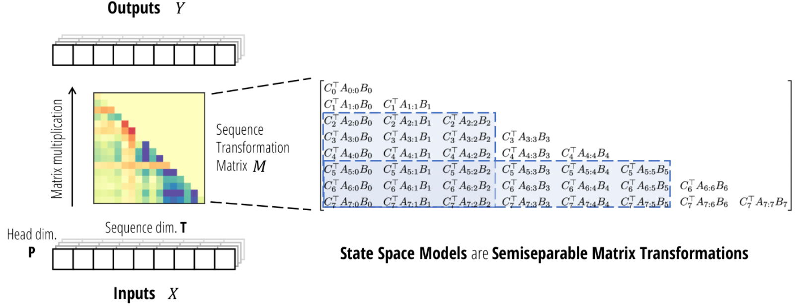
Figure 2: (**State Space Models are Semiseparable Matrices**.) As sequence transformations, state space models can be represented as a matrix transformation $M\in\mathbb{R}^{\mathtt{(T,T)}}$ acting on the sequence dimension $\mathtt{T}$ , sharing the same matrix for each channel in a head (Left). This matrix is a semiseparable matrix (Right), which is a rank-structured matrix where every submatrix contained on-and-below the diagonal (Blue) has rank at most $\mathtt{N}$ , equal to the SSM’s state dimension.

The reason Theorem 3.5 is important is that it will allow us to reduce the problem of efficient computation of SSMs (and other sequence models) into efficient algorithms for structured matrix multiplication. We briefly provide an overview and defer our main new algorithm to Section 6, after showing the equivalence of SSMs to other sequence models in Sections 4 and 5.

As previously defined, semiseparable matrices (i.e. rank-structured matrices) are a classical type of structured matrix:

(i)
They have compressed representations such as the SSS form which has only $O(\mathtt{T})$ instead of $O(\mathtt{T}^{2})$ parameters.
(ii)
They have fast algorithms operating directly on the compressed representation.

Furthermore, the parameterization and matrix multiplication cost can be tight in the semiseparable order.

Proposition 3.6 (Pernet et al. (2023)).

An $\mathtt{N}$ -SS matrix of size $\mathtt{T}$ can be represented in $O(\mathtt{NT})$ parameters and has matrix-vector multiplication in time and space $O(\mathtt{NT})$ .

For example, 1-SS matrices illustrate the essence of this connection. The matrix $M=\mathsf{1SS}(a)$ is defined by exactly $\mathtt{T}-1$ parameters $a_{0:\mathtt{T}-1}=a_{1},\dots,a_{\mathtt{T}-1}$ , and can be computed in $O(\mathtt{T})$ time by following the scalar recurrence (7).

Proposition 3.6 can be easily seen in the case of diagonal structured SSMs (S4D (Gu et al., 2022a)), simply by leveraging the state space model formulation (2) and unrolling the recurrence. We provide the formal tensor-contraction algorithm in (8), where the dimension $\mathtt{S}$ is equal to $\mathtt{T}$ $^{4}$ .

\begin{aligned}\displaystyle Z & \displaystyle=\mathsf{contract}(\mathtt{SP},\mathtt{SN}\to\mathtt{SPN})(X,B) & \displaystyle\mathtt{(S,P,N)} \\ \displaystyle H & \displaystyle=\mathsf{contract}(\mathtt{TSN},\mathtt{SPN}\to\mathtt{TPN})(L,Z) & \displaystyle\mathtt{(T,P,N)} \\ \displaystyle Y & \displaystyle=\mathsf{contract}(\mathtt{TN},\mathtt{TPN}\to\mathtt{TP})(C,H) & \displaystyle\mathtt{(T,P)}\end{aligned}

Here, $L\in\mathbb{R}^{(\mathtt{T},\mathtt{T})}$ is defined as $\mathsf{1SS}(A)$ , or in other words $L_{0:\mathtt{T},0:\mathtt{T}}=\mathsf{1SS}(A_{0:\mathtt{T}})$ for $i\in[\mathtt{N}]$ . This algorithm involves three steps corresponding to (2):

(i)
expanding the input $X$ by the input matrix $B$ (8a),
(ii)
unrolling independent scalar SSM recurrences (8b), and
(iii)
contracting the hidden state $H$ by the output matrix $C$ (8c).

Note that we have used the equivalence between scalar SSMs and 1-SS matrices in step (8b).

Remark 3.

We note that (8) is a special case of the Mamba (S6) model. however, a naive implementation is slow because of the expanded tensors $Z$ and $H$ of size $\mathtt{(T,P,N)}$ ; Gu & Dao (2023) introduced a hardware-aware implementation to avoid materializing these tensors.

Surprisingly, Theorem 3.5 and Proposition 3.6 immediately imply that all SSMs have the same asymptotic efficiency as algorithm (8).

Theorem 3.7.

Any state space model (Definition 2.2) of state size $\mathtt{N}$ on sequence length $\mathtt{T}$ can be computed in time $O(\mathtt{TN})$ (not accounting for potential preprocessing).

We note that this result is new to the structured SSM literature. In particular, given dense unstructured $A_{t}$ matrices, the total representation alone seems to be of size $O(\mathtt{TN}^{2})$ . Thus Theorem 3.7 states the non-trivial result that with a pre-processing step, even an unstructured SSM can be computed optimally efficiently, with upper bound matching the lower bound $O(\mathtt{TN})$ given by the size of $B$ and $C$ .

Remark 4.

Theorem 3.7 is perhaps not too surprising in light of the fact that almost all dense matrices over $\mathbb{R}^{\mathtt{(N,N)}}$ are diagonalizable over $\mathbb{C}$ , leading to the result that almost all dense real SSMs are equivalent to a diagonal complex SSM. This fact underlies the reason why diagonal SSMs are the most popular form of structured SSM (Gupta et al., 2022; Gu et al., 2022a; Smith et al., 2023). However, Theorem 3.7 implies the much stronger result for all real SSMs (not just the diagonalizable ones), as well as dense SSMs over other fields (including $\mathbb{C}$ itself).

In practice, efficiently computable SSMs still require additional structure on $A$ , particularly to avoid the expensive preprocessing step (which both has order $\mathtt{N}$ extra FLOPs and involves hardware-inefficient operations such as singular value decompositions). These structures are the focus of past work on structured SSMs (e.g. S4(D) and Mamba) as well as our new algorithms. In particular, when slightly stronger structure is imposed on $A$ , we will design very hardware-efficient algorithms through block decompositions of the SSM matrix $M=\mathsf{SSS}(A,B,C)$ in Section 6.

We note that there is another way to compute an SSM exposed by our new matrix point of view. A naive computation of the matrix SSM representation (3) involves simply materializing the sequence transformation matrix $M=\mathsf{SSS}(A,B,C)$ . This is a $\mathtt{(T,T)}$ matrix, and therefore this naive algorithm will scale quadratically in sequence length. However, when the sequence length $\mathtt{T}$ is short, this can actually be more efficient than the linear algorithm due to constant factors and the hardware-friendliness of the computation pattern (e.g. leveraging matrix-matrix multiplications). In fact, for a particular case of structured SSMs, this looks very similar to a quadratic attention computation (Section 5).

Many sequence models are explicitly motivated or defined as matrix sequence transformations – most notably Transformers, where the matrix mixer is the attention matrix. On the other hand, RNNs and SSMs have not previously been described in this way. By providing an explicit matrix transformation form of state space models, we reveal new ways of understanding and using them. From a computational perspective, any method of computing the forward pass of a state space model can be viewed as a matrix multiplication algorithm on semiseparable matrices. The semiseparable matrix perspective provides one lens into state space duality (SSD), where the dual modes respectively refer to a linear-time semiseparable matrix multiplication algorithm and quadratic-time naive matrix multiplication.

Moreover, leveraging the rich structure of semiseparable matrices can lead to even better algorithms and more insights (e.g. Sections 6 and B). In Section C.1, we describe some additional properties of semiseparable matrices.

In this section we revisit the linear attention framework from first principles. The main results in this section are a simple tensor-contraction-based proof of linear attention (Proposition 4.1), and our generalized abstraction of structured masked attention in Definition 4.2. We note that this section derives the main duality results from a different direction than state space models and can be read completely independently of Section 3.

•
Section 4.1 sets up our framework for variants of attention, with a particular focus on kernel attention and masked kernel attention.
•
Section 4.2 provides our first main attention result, a simple proof of linear attention through the lens of tensor contractions.
•
Section 4.3 defines structured masked attention, our generalization of prior attention variants through structured matrices.

The basic form of (single-head) attention is a map on three sequences of vectors $(Q,K,V)\mapsto Y$ .

\begin{aligned}\displaystyle Q & \displaystyle=\mathsf{input} & \displaystyle\mathtt{(T,N)} \\ \displaystyle K & \displaystyle=\mathsf{input} & \displaystyle\mathtt{(S,N)} \\ \displaystyle V & \displaystyle=\mathsf{input} & \displaystyle\mathtt{(S,P)} \\ \displaystyle G & \displaystyle=QK^{\top} & \displaystyle\mathtt{(T,S)} \\ \displaystyle M & \displaystyle=f(G) & \displaystyle\mathtt{(T,S)} \\ \displaystyle Y & \displaystyle=GV & \displaystyle\mathtt{(T,P)}\end{aligned}

We use “shape annotations” to indicate the dimensions of tensors, e.g. $Q\in\mathbb{R}^{\mathtt{(T,N)}}$ . In this general form, $\mathtt{S}$ and $\mathtt{T}$ represent source and target sequence lengths, $\mathtt{N}$ represents the feature dimension, and $\mathtt{P}$ represents the head dimension.

The most common variant of softmax attention uses a softmax activation $f=\mathsf{softmax}$ to normalize the rows of the $G$ matrix.

Our treatment is motivated by the most important case of self-attention, where

(i)
the source and target sequences are the same (i.e. $\mathtt{S}=\mathtt{T}$ ),
(ii)
usually the feature and head dimensions are the same (i.e. $\mathtt{N}=\mathtt{P}$ ),
(iii)
and $Q,K,V$ are generated by linear projections on the same input vector ( $Q=W_{Q}\cdot X,K=W_{K}\cdot X,V=W_{V}\cdot X$ ).

However, our presentation abstracts away these choices and begins from the $Q,K,V$ matrices.

Remark 5.

Our focus is on the self-attention case with equal head and feature dimensions (i.e. $\mathtt{S}=\mathtt{T}$ and $\mathtt{N}=\mathtt{P}$ ), which should be used as the running example. We define the general formulation of attention not only so that our framework captures variants such as cross-attention, but also because separating the notation for dimensions (e.g. $\mathtt{S}$ and $\mathtt{T}$ ) makes the contraction notation proofs of our main results in this section more clear.

Remark 6.

While attention is usually framed as an operation on these three inputs $Q,K,V$ which are viewed symmetrically, the input and output dimensions in (9) indicate otherwise. In particular, the feature dimension $\mathtt{N}$ is not present in the output; therefore in the case when $\mathtt{S}=\mathtt{T}$ (e.g. self-attention), we view $V$ as the main input, so that (9) defines a proper sequence transformation $V\mapsto Y$ (Definition 2.1).

The step where the softmax function is applied to the Gram matrix $G$ can be decomposed into two parts:

1.
Exponentiating the $G$ matrix.
2.
Normalizing the $G$ matrix on the $\mathtt{S}$ axis.

We can ignore the normalization term for now, as it amounts to simply passing in $V=1$ and dividing (we revisit this in Section 7.3). The exponentiation term can be viewed as a kernel transformation: there is an (infinite-dimensional) feature map $\varphi$ such that $\exp(QK^{\top})=\varphi(Q)\varphi(K)^{\top}$ . By abstracting away the feature map into the definition of $Q$ and $K$ itself (i.e. define $Q,K$ as the post-transformed versions), we can ignore the softmax transformation, and assume that $Q,K$ are arbitrarily generated by kernel feature maps and potentially $\mathtt{N}\neq\mathtt{P}$ .

Many instantiations of kernel attention have been proposed, including:

•
The original Linear Attention (Katharopoulos et al., 2020) defines the kernel feature map as an arbitrary pointwise activation function, such as $x\mapsto 1+\mathsf{elu}(x)$ .
•
Random Feature Attention (RFA) (Peng et al., 2021) chooses the kernel feature map to approximate softmax attention (i.e. the $\exp$ feature map) using the random Fourier feature approximation of Gaussian kernels (Rahimi & Recht, 2007). This involves random projections (i.e. multiplying $Q$ and $K$ by a random projection $W$ and applying the activation $x\mapsto(\cos(x),\sin(x))$ .
•
Performer (Choromanski et al., 2021) proposes the fast attention via positive orthogonal random features (FAVOR+). The positive random features (PRF) part chooses the kernel feature map to be a random projection followed by the feature map $x\mapsto 2^{-1/2}(\exp(x),\exp(-x))$ . This choice is motivated so that the kernel elements are positive-valued and provably approximates the softmax attention. [It also proposes choosing the random projections in orthogonal directions, which we do not consider.]
•
cosFormer (Qin et al., 2022a) augment RFA with a cosine reweighting mechanism that incorporates positional information to emphasize locality. This effectively passes $Q_{t},K_{t}$ through the feature map $x\mapsto(x\cos(\pi t/2T),\sin(\pi t/2T))$ .
•
Linear Randomized Attention (Zheng et al., 2022) generalize RFA from the perspective of importance sampling, and generalize it to provide better estimates of the full softmax kernel (rather than just the $\exp$ -transformed numerator).

Other related attention variants include Linformer (Wang et al., 2020) and Nyströformer (Xiong et al., 2021), which both use low-rank approximations of the attention matrix $M$ (and are thus compatible with equation (9)), through random projections (Johnson-Lindenstrauss) and kernel approximation (the Nyström method) respectively.

Let $L$ be a mask of shape $\mathtt{(T,S)}$ . Most commonly, in the autoregressive self-attention case when $\mathtt{S}=\mathtt{T}$ , $L$ may be a lower-triangular matrix of $1$ ’s representing a causal mask. Besides enforcing causality, many other types of masks can be applied – in particular various sparsity patterns such as banded, dilated, or block diagonal – which are motivated by reducing the complexity of dense attention.

Masked attention is usually written in matrix notation as

y=(L\circ(QK^{\top}))\cdot V.

More precisely, with shape annotations and breaking this down into the precise sequence of computations:

\begin{aligned}\displaystyle G & \displaystyle=QK^{\top} & \displaystyle\mathtt{(T,S)} \\ \displaystyle M & \displaystyle=G\circ L & \displaystyle\mathtt{(T,S)} \\ \displaystyle Y & \displaystyle=MV & \displaystyle\mathtt{(T,P)}\end{aligned}

Our improved derivation of attention variants in this section starts by noticing that this formula can be written as a single contraction:

Y=\mathsf{contract}(\mathtt{TN},\mathtt{SN},\mathtt{SP},\mathtt{TS}\to\mathtt{TP})(Q,K,V,L)

and the algorithm in (11) can be reframed as computing (12) by a particular ordering of pairwise contractions

\begin{aligned}\displaystyle G & \displaystyle=\mathsf{contract}(\mathtt{TN,SN}\to\mathtt{TS})(Q,K) & & \displaystyle\qquad\mathtt{(T,S)} \\ \displaystyle M & \displaystyle=\mathsf{contract}(\mathtt{TS,TS}\to\mathtt{TS})(G,L) & & \displaystyle\qquad\mathtt{(T,S)} \\ \displaystyle Y & \displaystyle=\mathsf{contract}(\mathtt{TS,SP}\to\mathtt{TP})(M,V) & & \displaystyle\qquad\mathtt{(T,P)}\end{aligned}

Linear attention, and many other variants of efficient attention, is often motivated by changing the order of matrix associativity in the core attention computation $(QK^{\top})V=Q(K^{\top}V)$ . However when the mask is added, the derivation is somewhat less straightforward (for example, the original paper (Katharopoulos et al., 2020) and variants (Sun et al., 2023) state the formula without proof).

Roughly, the linear attention method claims that the following formula is equivalent to (10), which must be verified by expanding the sum and tracking indices carefully.

Y=Q\cdot\mathsf{cumsum}(K^{\top}V)

Proposition 4.1 ((Katharopoulos et al., 2020)).

Autoregressive kernel attention, i.e. masked kernel attention with the causal mask, can be computed in $O(T)$ time by a recurrence taking constant time per step.

We present a simple and rigorous derivation of linear attention that will also immediately reveal how to generalize it. The main idea is to perform the contraction (12) in an alternate order. We avoid ambiguous matrix notation and work directly with contraction notation:

\begin{aligned}\displaystyle Z & \displaystyle=\mathsf{contract}(\mathtt{SP},\mathtt{SN}\to\mathtt{SPN})(V,K) & \displaystyle\mathtt{(S,P,N)} \\ \displaystyle H & \displaystyle=\mathsf{contract}(\mathtt{TS},\mathtt{SPN}\to\mathtt{TPN})(L,Z) & \displaystyle\mathtt{(T,P,N)} \\ \displaystyle Y & \displaystyle=\mathsf{contract}(\mathtt{TN},\mathtt{TPN}\to\mathtt{TP})(Q,H) & \displaystyle\mathtt{(T,P)}\end{aligned}

Intuitively, we interpret this contraction order as follows.

The first step (15a) performs an “expansion” into more features, by a factor of the feature dimension $\mathtt{N}$ . The third step (15c) contracts the expanded feature dimension away. If $K$ is viewed as the input (Remark 6), then $V$ and $Q$ perform the expansion and contraction, respectively.

The second step is the most critical, and explains the linear part of linear attention. First notice that (15b) is just a direct matrix multiplication by $L$ (since the $\mathtt{(P,N)}$ axes can be flattened). Also note that this is the only term that involves both $\mathtt{T}$ and $\mathtt{S}$ axes, hence should have $\Omega(\mathtt{TS})$ complexity (i.e. quadratic in sequence length). However, when the mask $L$ is the standard causal attention mask (lower triangular $1$ ’s), matrix-vector multiplication by $L$ is identical to a feature-wise cumulative sum

\displaystyle y=\begin{bmatrix}1\\ \vdots&\ddots\\ 1&\dots&1\end{bmatrix}x\quad\iff\quad\begin{aligned} y_{0}&=x_{0}\\ y_{t}&=y_{t-1}+x_{t}\end{aligned}.

With the tensor contraction perspective of masked attention (15), we can immediately see that the crux of the original linear attention is the fact that matrix-vector multiplication by the causal mask is equivalent to the cumulative sum operator.

However, we observe that there is no reason the attention mask has to be all $1$ ’s. All that is necessary for linear attention to be fast is for $L$ to be a structured matrix, which by definition are those that have fast matrix multiplication (Section 2.3). In particular, we can use any mask matrix $L$ that has sub-quadratic (ideally linear) matrix-vector multiplication, which would have the same complexity as standard linear attention by speeding up the bottleneck equation (15b).

Definition 4.2.

Structured masked attention (SMA) (or structured attention for short) is defined as a function on queries/keys/values $Q,K,V$ as well as any structured matrix $L$ (i.e. has sub-quadratic matrix multiplication), through the 4-way tensor contraction

\displaystyle Y=\mathsf{contract}(\mathtt{TN},\mathtt{SN},\mathtt{SP},\mathtt{TS}\to\mathtt{TP})(Q,K,V,L).

The SMA quadratic mode algorithm is the sequence of pairwise contractions defined by (13), which corresponds to the standard (masked) attention computation.

The SMA linear mode algorithm is the sequence of pairwise contractions defined by (15), where step (15b) is optimized through the subquadratic structured matrix multiplication.

We can instantiate structured masked attention to any given class of matrix structure. Some examples include (Figure 3):

•
Linear attention uses a causal mask.
•
RetNet (Sun et al., 2023) uses a decay mask $L_{ij}=\gamma^{i-j}\cdot\mathbb{I}[j\geq i]$ for some decay factor $\gamma\in[0,1]$ .
•
The decay mask could be generalized to a Toeplitz matrix $L_{ij}=\alpha_{i-j}$ for some learnable (or input-dependent) set of parameters $\alpha\in\mathbb{R}^{\mathtt{T}}$ . This can be interpreted as a form of relative positional encoding, reminiscent of other methods such as AliBi (Press et al., 2022) but multiplicative instead of additive.
•
Another variant could use a Fourier matrix $L_{ij}=\omega^{ij/\mathtt{T}}$ to encode positional structure a different way.

In Section 5, we consider semiseparable SMA, which defines our main SSD model.

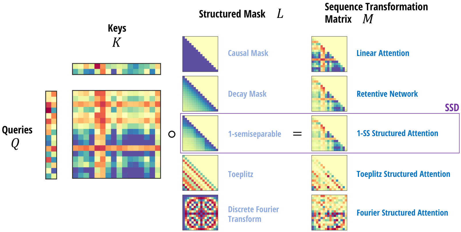
Figure 3: (**Structured Masked Attention**.) SMA constructs a masked attention matrix $M=QK^{\top}\circ L$ for any structured matrix $L$ , which defines a matrix sequence transformation $Y=MV$ . All instances of SMA have a dual subquadratic form induced by a different contraction ordering, combined with the efficient structured matrix multiplication by $L$ . Previous examples include Linear Attention (Katharopoulos et al., 2020) and RetNet (Sun et al., 2023). Beyond SSD (1-semiseparable SMA), the focus of this paper, many other potential instantiations of structured attention are possible.

Standard (masked kernel) attention is often conflated between a function and an algorithm. Separating this distinction presents a clear way to understand different variants of attention.

•
We view masked attention as a particular function (12).
•
The standard quadratic attention computation (13) can be viewed as an algorithm to compute the function.
•
Linear attention (15) is an alternate algorithm to compute the same function.

Moreover, in this case

•
The masked attention function is simply a particular contraction on four terms.
•
The quadratic and linear attention algorithms are simply two different orders to perform the contractions.

It is known that contraction orderings can make large differences in computation complexity, leading to the quadratic vs. linear split. Just as state space models are a transformation that can be computed in multiple ways, with dual quadratic vs. linear forms (Section 3.4), linear attention has a similar duality that results from two contraction orders. In fact, these turn out to be different perspectives on the same underlying duality, which we make explicit in Section 5.

In Sections 3 and 4, we defined structured state space models and structured attention, discussed their properties, and showed that they both have a quadratic algorithm and a linear algorithm. This section connects them together. Our main result is showing that a particular case of structured state space models coincides with a particular case of structured attention, and that the linear-time SSM algorithm and quadratic-time kernel attention algorithm are dual forms of each other.

•
Section 5.1 specializes state space models to scalar structure, where the naive quadratic computation can be seen as an instance of kernel attention.
•
Section 5.2 specializes structured masked attention to semiseparable SMA, which characterizes masked attention with efficient autoregression.
•
Section 5.3 summarizes the connection between structured masked attention and structured state space models, termed structured state space duality.

In Section 3 we showed that state space models are equivalent to semiseparable matrix transformations, resulting in both a linear recurrent form and quadratic naive form.

Recall that SSMs are defined by $y=\mathsf{SSM}(A,B,C)(x)$ , and the matrix form of SSMs uses the SSS (sequentially semiseparable) representation $M=\mathsf{SSS}(A,B,C)$ where $M_{ji}=C_{j}^{\top}A_{j:i}B_{i}$ (equation (3)).

Now let us consider the case where $A_{j}$ is simply a scalar; in other words, an instantiation of a structured SSM where the $A$ matrices are extremely structured: $A=aI$ for scalar $a$ and identity matrix $I$ . Then we can rearrange

\displaystyle M_{ji}=A_{j:i}\cdot(C_{j}^{\top}B_{i}).

And this can be vectorized into

\begin{aligned}\displaystyle L & \displaystyle\coloneqq\mathsf{1SS}(a)\end{aligned}

\begin{aligned}\displaystyle M & \displaystyle=L\circ(CB^{\top})\end{aligned}

where $B,C\in\mathbb{R}^{\mathtt{(T,N)}}$ .

Using this formulation, the full output $Y=MX$ is computed precisely as

\begin{aligned}\displaystyle G & \displaystyle=\mathsf{contract}(\mathtt{TN,SN\to TS})(C,B) & & \displaystyle\mathtt{(T,S)} \\ \displaystyle M & \displaystyle=\mathsf{contract}(\mathtt{TS,TS\to TS})(G,L) & & \displaystyle\mathtt{(T,S)} \\ \displaystyle Y & \displaystyle=\mathsf{contract}(\mathtt{TS,SP\to TP})(M,X) & & \displaystyle\mathtt{(T,P)}\end{aligned}

where $\mathtt{S}=\mathtt{T}$ . But this is exactly the same as original definition of masked kernel attention definition (13)!

Therefore, as alluded to in Section 3.4, naively computing the scalar structured SSM—by materializing the semiseparable matrix $M$ and performing quadratic matrix-vector multiplication—is exactly the same as quadratic masked kernel attention.

Structured masked attention allows for the use of any structured mask $L$ . When $L$ is the causal mask, it is standard linear attention. Note that the causal mask is $L=\mathsf{SS}(1_{T})$ , i.e. the $1$ -SS mask is generated by $a_{t}=1$ in definition (6). This motivates generalizing $L$ to the class of 1-semiseparable masks, or 1-semiseparable structured masked attention (1-SS SMA), where the $\mathsf{cumsum}$ in linear attention’s recurrence is replaced by a more general recurrence – the scalar SSM scan, i.e. 1-semiseparable matrix multiplication (Section 3.2.2).

Finally, the most important reason we consider 1-semiseparable SMA is because the linear form for computing it is a special case of diagonal state space model. The linear form of SMA is algorithm (15), where the bottleneck step (15b) can be viewed as matrix multiplication by the 1-SS mask. In Section 3, we also wrote out the computation for a diagonal SSM (8), where the bottleneck step (8b) is a scalar SSM recurrence which is equivalent to 1-SS multiplication. The only difference is that (8b) has an extra $\mathtt{N}$ dimension in $L$ , because the matrix $A$ is a diagonal matrix of size $\mathtt{N}$ . This $\mathtt{N}$ dimension would disappear if all diagonal entries of $A$ are the same, which results in Corollary 5.1.

Corollary 5.1.

1-SS SMA (masked attention with 1-semiseparable structured matrices $L$ ) (15) is a special case of a diagonal SSM (8) where the diagonal matrix is a scalar multiple of the identity.

While Corollary 5.1 says that 1-SS SMA has an efficient recurrent form, we can also show a converse result that characterizes which instances of SMA has efficient autoregression.

Theorem 5.2.

For any instantiation of structured masked attention (Definition 4.2) that is an autoregressive process with bounded order, the structured mask $L$ must be a semiseparable matrix.

In other words, efficient autoregressive attention is general semiseparable SMA. Theorem 5.2 is proved in Section C.2.

Remark 7.

While 1-semiseparable SMA is a special case of a state space model, general semiseparable SMA is strictly more expressive than 1-SS SMA, and cannot be described by a standard SSM. However, the semiseparable multiplication by $L$ and the linear form of SMA (equation (15a)) each involve an expansion and contraction step, and can be absorbed into a similar instance of 1-SS SMA with a single (larger) expansion.

In summary, 1-semiseparable structured attention is the most important case of SMA, because it is:

•
a natural generalization of linear attention with an input-dependent recurrence.
•
the simplest case of general semiseparable attention, which is equivalent to efficient autoregressive attention.
•
a special case of a diagonal state space model.

To summarize our results:

•
Structured state-space models (Section 3) are a model usually defined through a linear-time recurrence. However, by expanding the matrix formulation characterizing its linear sequence-to-sequence transformation, one can derive a quadratic form.
•
Attention variants (Section 4) are a model defined through quadratic-time pairwise interactions. However, by viewing it as a four-way tensor contraction and reducing in a different order, one can derive a linear form.
•
A natural special case of each one – more precisely, state space models with scalar-identity structure on the $A$ matrices, and structured masked attention with 1-semiseparable structure on its $L$ mask – are duals of each other with the exact same linear and quadratic forms.

Figure 4 summarizes the duality between these two representations.

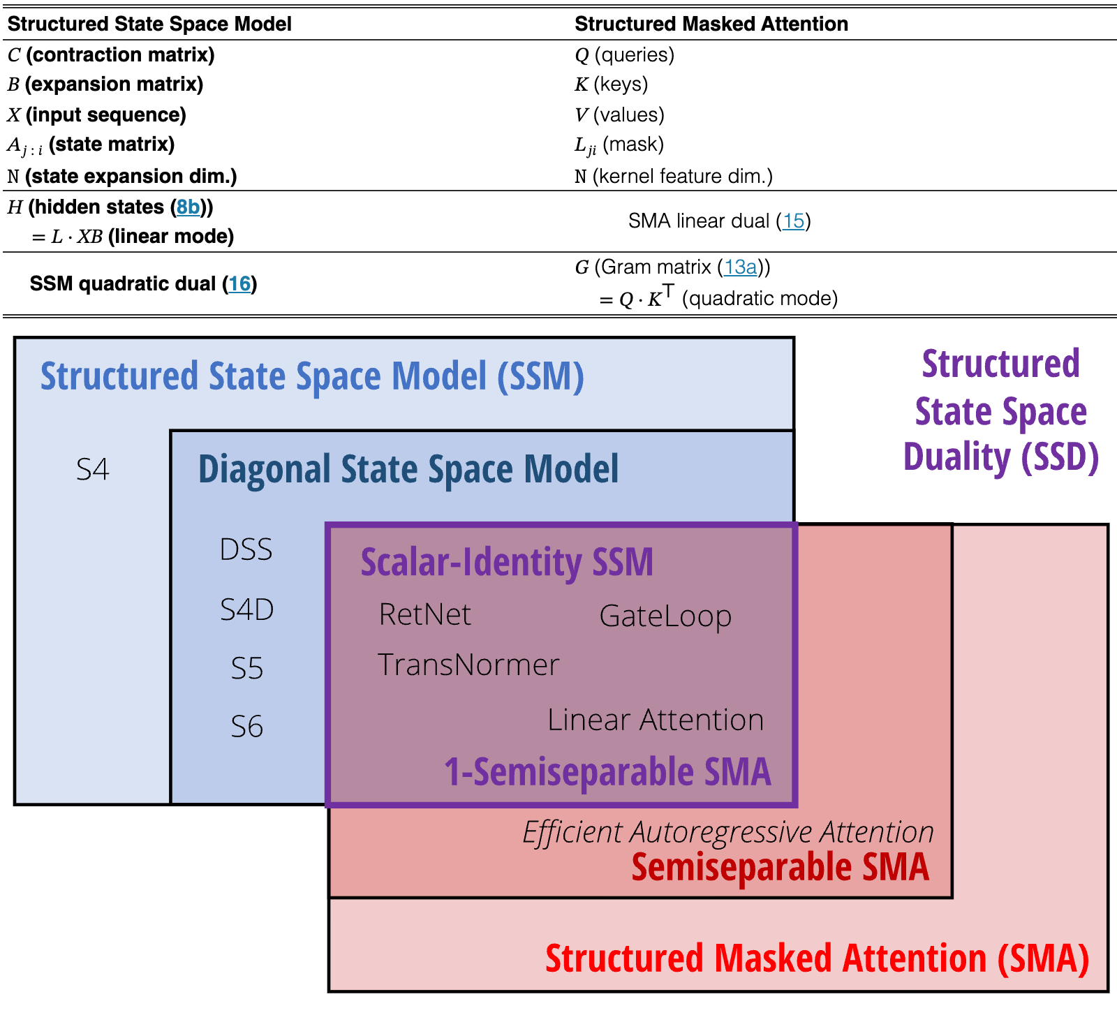
Figure 4: (**Structured State Space Duality**.) State space duality describes the close relationship between state space models and masked attention. (Left) General SSMs and SMA both possess linear and quadratic forms, with direct analogs in notation. (Right) SSMs and SMA intersect at a large class of state space dual models (SSD) which capture many sequence models as special cases.

An extended related work and discussion (Section 10) describes the relationship between SSD and general SSMs / attention in more detail.

The benefits of developing the theoretical SSD framework between SSMs, attention, and structured matrices lies in using the connections to improve the models and algorithms. In this section, we show how various algorithms for computing SSD models efficiently can be derived from various algorithms for computing structured matrix multiplication.

Our main computational result is an algorithm for computing SSD models that combines both the linear (recurrent) mode and quadratic (attention) mode. This algorithm is as computation efficient as SSMs (linear scaling in sequence length) and as hardware-friendly as attention (primarily uses matrix multiplications).

Theorem 6.1.

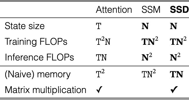
Consider an SSD model with state expansion factor $\mathtt{N}$ and head dimension $\mathtt{P}=\mathtt{N}$ . There exists an algorithm for computing the model on any input $X\in\mathbb{R}^{\mathtt{(T,P)}}$ which only requires $O(\mathtt{TN}^{2})$ training FLOPs, $O(\mathtt{TN})$ inference FLOPs, $O(\mathtt{N}^{2})$ inference memory, and whose work is dominated by matrix multiplications.

Note that all of these bounds are tight, because a state space model with state expansion $\mathtt{N}$ operating on a head size of $\mathtt{N}$ has total state size $\mathtt{N}^{2}$ (yielding the lower bounds for training and inference FLOPs of $O(\mathtt{TN}^{2})$ and $O(\mathtt{N}^{2})$ respectively). Furthermore the input $X$ itself has $\mathtt{TN}$ elements, yielding the memory lower bound.

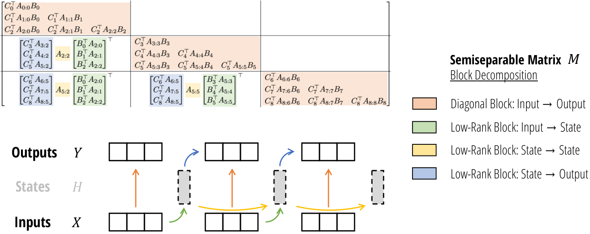
The main idea behind Theorem 6.1 is once again viewing the problem of computing a state space model as a semiseparable matrix multiplication, but leveraging its structure in a new way. Instead of computing the whole matrix in either recurrent or attention mode, we perform a block decomposition of the matrix. The diagonal blocks can be computed using the dual attention mode, which can be efficiently done with matrix multiplications, while the off-diagonal blocks can be factored by the rank-structure of semiseparable matrices and reduced to a smaller recurrence. We highlight that Section 6.2 provides a self-contained implementation of the SSD algorithm. Compared to the general selective SSM of Gu & Dao (2023), this implementation is much simpler, and relatively efficient even in native PyTorch without requiring special low-level kernels.

To begin, we partition the matrix $M$ into a $\frac{\mathtt{T}}{\mathtt{Q}}\times\frac{\mathtt{T}}{\mathtt{Q}}$ grid of submatrices of size $\mathtt{Q}\times\mathtt{Q}$ , for some block size $\mathtt{Q}$ . Note that the off-diagonal blocks are low-rank by the defining property of semiseparable matrices (Definition 3.1). $^{5}$

\begin{aligned}\displaystyle\text{(Block Decomposition)}\quad M & \displaystyle=\begin{bmatrix}M^{(0,0)}\\ M^{(1,0)}&M^{(1,1)}\\ \vdots&\vdots&\ddots\\ M^{(\mathtt{T}/\mathtt{Q}-1,0)}&M^{(\mathtt{T}/\mathtt{Q}-1,1)}&\dots&M^{(\mathtt{T}/\mathtt{Q}-1,\mathtt{T}/\mathtt{Q}-1)}\\ \end{bmatrix}\end{aligned}

\begin{aligned}\displaystyle\text{(Diagonal Block)}\quad M^{(j,j)} & \displaystyle=\mathsf{SSM}(A_{j\mathtt{Q}:(j+1)\mathtt{Q}},B_{j\mathtt{Q}:(j+1)\mathtt{Q}},C_{j\mathtt{Q}:(j+1)\mathtt{Q}})\end{aligned}

\begin{aligned}\displaystyle\text{(Low-Rank Block)}\quad M^{(j,i)} & \displaystyle=\begin{bmatrix}C_{j\mathtt{Q}}^{\top}A_{j\mathtt{Q}:j\mathtt{Q}-1}\\[1.0pt] \vdots\\[1.0pt] C_{(j+1)\mathtt{Q}-1}^{\top}A_{(j+1)\mathtt{Q}-1:j\mathtt{Q}-1}\end{bmatrix}A_{j\mathtt{Q}-1:(i+1)\mathtt{Q}-1}\begin{bmatrix}B_{i\mathtt{Q}}^{\top}A_{(i+1)\mathtt{Q}-1:i\mathtt{Q}}\\[1.0pt] \vdots\\[1.0pt] B_{(i+1)\mathtt{Q}-1}^{\top}A_{(i+1)\mathtt{Q}-1:(i+1)\mathtt{Q}-1}\end{bmatrix}^{\top}\end{aligned}

This is easiest illustrated through an example, e.g. for $\mathtt{T}=9$ and decomposing into chunks of length $\mathtt{Q}=3$ . The shaded cells are low-rank factorizations of the off-diagonal blocks of the semiseparable matrix.

Fromherewecanreducetheproblemintothesetwoparts.Thesecanalsobeinterpretedasdividingtheoutputofa``chunk ′ ′ y_jQ:(j+1)Q $intotwocomponents:theeffectofinputswithinthechunk$ x_jQ:(j+1)Q $,andtheeffectofinputsbeforethechunk$ x_0:jQ.

The diagonal blocks are easy to handle, because they are simply self-similar problems of a smaller size. The $j$ -th block represents computing the answer $\mathsf{SSM}(A_{R},B_{R},C_{R})(x_{R})$ for the range $R=j\mathtt{Q}:(j+1)\mathtt{Q}=(j\mathtt{Q},j\mathtt{Q}+1,\dots,j\mathtt{Q}+\mathtt{Q}-1)$ . The key is that this block can be computed using any desired method. In particular, for small chunk lengths $\mathtt{Q}$ , this problem is computed more efficiently using the dual quadratic SMA form. Additionally, the chunks can be computed in parallel.

These subproblems can be interpreted as: what is the output per chunk supposing that the initial state (to the chunk) is $0$ . In other words for chunk $j$ , this computes the correct outputs taking into account only the chunk inputs $x_{j\mathtt{Q}:(j+1)\mathtt{Q}}$ .

The low-rank factorizations consist of 3 terms, and there are correspondingly three pieces of the computation. In this factorization, we will use the terminology

•
The terms like $\begin{bmatrix}B_{0}^{\top}A_{2:0}\\[1.0pt] B_{1}^{\top}A_{2:1}\\[1.0pt] B_{2}^{\top}A_{2:2}\end{bmatrix}^{\top}$ are called the right factors or $B$ -block-factors.
•
The terms like $A_{5:2}$ are called the center factors or $A$ -block-factors.
•
The terms like $\begin{bmatrix}C_{6}^{\top}A_{6:5}\\[1.0pt] C_{7}^{\top}A_{7:5}\\[1.0pt] C_{8}^{\top}A_{8:5}\end{bmatrix}$ are called the left factors or $C$ -block-factors.

This step computes the multiplication by the right $B$ -block-factors of the low-rank factorization. Note that for each chunk, this is a $(\mathtt{N},\mathtt{Q})$ by $(\mathtt{Q},\mathtt{P})$ matrix multiplication, where $\mathtt{N}$ is the state dimension and $P$ is the head dimension. The result is a $(\mathtt{N},\mathtt{P})$ tensor for each chunk, which has the same dimensionality as the expanded hidden state $h$ .

This can be interpreted as: what is the final state per chunk supposing that the initial state (to the chunk) is $0$ . In other words this computes $h_{j\mathtt{Q}+\mathtt{Q}-1}$ assuming that $x_{0:j\mathtt{Q}}=0$ .

This step computes the effect of the center $A$ -block-factors terms in the low-rank factorization. In the previous step, the final states per chunk have total shape $\mathtt{(\mathtt{T}/\mathtt{Q},\mathtt{N},\mathtt{P})}$ . This is now multiplied by a 1-SS matrix generated by $A_{2\mathtt{Q}-1:\mathtt{Q}-1}^{\times},A_{3\mathtt{Q}-1:2\mathtt{Q}-1}^{\times},\dots,A_{\mathtt{T}-1:\mathtt{T}-\mathtt{Q}-1}^{\times}$ .

This step can be computed by any algorithm for computing 1-SS multiplication (also known as the scalar SSM scan or cumprodsum operator).

This can be interpreted as: what is the actual final state per chunk taking into account all previous inputs; in other words, this computes the true hidden state $h_{j\mathtt{Q}}$ taking into account all of $x_{0:(j+1)\mathtt{Q}}$ .

This step computes the multiplication by the left $C$ -block-factors of the low-rank factorization. For each chunk, this can be represented by a matrix multiplication $\mathsf{contract}(\mathtt{QN,NP\to QP})$ .

This can be interpreted as: what is the output per chunk taking into account the correct initial state $h_{j\mathtt{Q}-1}$ , and supposing the inputs $x_{j\mathtt{Q}:(j+1)\mathtt{Q}}$ are $0$ . In other words for chunk $j$ , this computes the correct outputs taking into account only the prior inputs $x_{0:j\mathtt{Q}}$ .

[!t]

def segsum(x):

"""Naive segment sum calculation. exp(segsum(A)) produces a 1-SS matrix,

which is equivalent to a scalar SSM."""

T = x.size(-1)

x_cumsum = torch.cumsum(x, dim=-1)

x_segsum = x_cumsum[…, :, None] - x_cumsum[…, None, :]

mask = torch.tril(torch.ones(T, T, device=x.device, dtype=bool), diagonal=0)

x_segsum = x_segsum.masked_fill(~mask, -torch.inf)

return x_segsum

def ssd(X, A, B, C, block_len=64, initial_states=None):

"""

Arguments:

X: (batch, length, n_heads, d_head)

A: (batch, length, n_heads)

B: (batch, length, n_heads, d_state)

C: (batch, length, n_heads, d_state)

Return:

Y: (batch, length, n_heads, d_head)

"""

assert X.dtype == A.dtype == B.dtype == C.dtype

assert X.shape[1] % block_len == 0

# Rearrange into blocks/chunks

X, A, B, C = [rearrange(x, "b (c l) … -> b c l …", l=block_len) for x in (X, A, B, C)]

A = rearrange(A, "b c l h -> b h c l")

A_cumsum = torch.cumsum(A, dim=-1)

# 1. Compute the output for each intra-chunk (diagonal blocks)

L = torch.exp(segsum(A))

Y_diag = torch.einsum("bclhn,bcshn,bhcls,bcshp->bclhp", C, B, L, X)

# 2. Compute the state for each intra-chunk

# (right term of low-rank factorization of off-diagonal blocks; B terms)

decay_states = torch.exp((A_cumsum[:, :, :, -1:] - A_cumsum))

states = torch.einsum("bclhn,bhcl,bclhp->bchpn", B, decay_states, X)

# 3. Compute the inter-chunk SSM recurrence; produces correct SSM states at chunk boundaries

# (middle term of factorization of off-diag blocks; A terms)

if initial_states is None:

initial_states = torch.zeros_like(states[:, :1])

states = torch.cat([initial_states, states], dim=1)

decay_chunk = torch.exp(segsum(F.pad(A_cumsum[:, :, :, -1], (1, 0))))

new_states = torch.einsum("bhzc,bchpn->bzhpn", decay_chunk, states)

states, final_state = new_states[:, :-1], new_states[:, -1]

# 4. Compute state -> output conversion per chunk

# (left term of low-rank factorization of off-diagonal blocks; C terms)

state_decay_out = torch.exp(A_cumsum)

Y_off = torch.einsum(’bclhn,bchpn,bhcl->bclhp’, C, states, state_decay_out)

# Add output of intra-chunk and inter-chunk terms (diagonal and off-diagonal blocks)

Y = rearrange(Y_diag+Y_off, "b c l h p -> b (c l) h p")

return Y, final_state

Full PyTorch example of the state space dual (SSD) model.

Figure 5: (**SSD Algorithm**.) By using the matrix transformation viewpoint of state space models to write them as semiseparable matrices (Section 3), we develop a more hardware-efficient computation of the SSD model through a block-decomposition matrix multiplication algorithm. The matrix multiplication also has an interpretation as a state space model, where blocks represent chunking the input and output sequence. Diagonal blocks represent intra-chunk computations and the off-diagonal blocks represent inter-chunk computations, factored through the SSM’s hidden state.

We define the notation $\mathsf{BMM}(\mathtt{B},\mathtt{M},\mathtt{N},\mathtt{K})$ to define a batched matrix multiplication $\mathsf{contract}(\mathtt{\mathtt{MK},\mathtt{KN}\to\mathtt{MN}})$ with batch dimension $\mathtt{B}$ . From this notation we can infer three aspects of the efficiency:

•
Computation cost: total of $O(\mathtt{BMNK})$ FLOPs.
•
Memory cost: total of $O(\mathtt{B}(\mathtt{MK}+\mathtt{KN}+\mathtt{MN}))$ space.
•
Parallelization: larger $\mathtt{M},\mathtt{N},\mathtt{K}$ terms can leverage specialized matrix multiplication units on modern accelerators.

The cost of the quadratic SMA computation consists of three steps (equation (16)):

•
Computing the kernel matrix $C^{\top}B$ , which has cost $\mathsf{BMM}(\mathtt{T}/\mathtt{Q},\mathtt{Q},\mathtt{Q},\mathtt{N})$ .
•
Multiplying by the mask matrix, which is an elementwise operation on tensors of shape $(\mathtt{T}/\mathtt{Q},\mathtt{Q},\mathtt{Q})$ .
•
Multiplying by the $X$ values, which has cost $\mathsf{BMM}(\mathtt{T}/\mathtt{Q},\mathtt{Q},\mathtt{P},\mathtt{N})$

This step is a single matrix multiplication with cost $\mathsf{BMM}(\mathtt{T}/\mathtt{Q},\mathtt{N},\mathtt{P},\mathtt{Q})$ .

This step is a scalar SSM scan (or 1-SS multiplication) of length $\mathtt{T}/\mathtt{Q}$ on $(\mathtt{N},\mathtt{P})$ independent channels. The work of this scan is $\mathtt{TNP}/\mathtt{Q}$ , which is negligible compared to the other factors.

Note that because of the blocking which reduces the length of the sequence from $\mathtt{T}$ to $\mathtt{T}/\mathtt{Q}$ , this scan has $\mathtt{Q}$ times smaller cost than a pure SSM scan (e.g. the selective scan of Mamba). Thus we observe that on most problem lengths, other algorithms (Appendix B) may be more efficient or much easier to implement without a significant slowdown. For example, a naive implementation of this via 1-SS matrix multiplication has cost $\mathsf{BMM}(1,\mathtt{T}/\mathtt{Q},\mathtt{NP},\mathtt{T}/\mathtt{Q})$ , which is much easier to implement and can be more efficient than a naive recurrence/scan implementation.

This step is a single matrix multiplication with cost $\mathsf{BMM}(\mathtt{T}/\mathtt{Q},\mathtt{Q},\mathtt{P},\mathtt{N})$ .

If we set $\mathtt{N}=\mathtt{P}=\mathtt{Q}$ (in other words the state dimension, head dimension, and chunk length are equal), then all BMM terms above become $\mathsf{BMM}(\mathtt{T}/\mathtt{N},\mathtt{N},\mathtt{N},\mathtt{N})$ . The computational chacteristics of this are:

•
Total FLOP count of $O(\mathtt{TN}^{2})$ .
•
Total memory of $O(\mathtt{TN})$ .
•
The work consists primarily of matrix multiplications on matrices of shape $(\mathtt{N},\mathtt{N})$ .

Notice that the memory consumption is tight; the inputs and outputs $x,y$ have shape $(\mathtt{T},\mathtt{P})=(\mathtt{T},\mathtt{N})$ . Meanwhile the flop count reflects an extra factor of $\mathtt{N}$ , which is cost incurred by the autoregressive state size and is common to all models.

Aside from the matmuls, there is a scalar SSM scan on $\mathtt{NP}=\mathtt{N}^{2}$ features and sequence length $\mathtt{T}/\mathtt{Q}$ . This has cost $O(\mathtt{T}/\mathtt{Q}\mathtt{N}^{2})$ FLOPs and $O(\log(\mathtt{T}/\mathtt{Q}))$ depth. Although it does not use matrix multiplications, it is still parallelizable and the total work done is negligible compared to the other steps; this has a negligible cost in our GPU implementation.

Quadratic attention is also very hardware efficient by only leveraging matrix multiplications, but has $\mathtt{T}^{2}N$ total FLOPs. Its slower computation speed at both training and inference can directly be seen as a consequence of having a larger state size – standard attention has a state size scaling with sequence length $\mathtt{T}$ because it caches its history and does not compress its state.

Linear SSMs have $\mathtt{TNP}=\mathtt{TN}^{2}$ total FLOPs, which is the same as SSD. However, a naive implementation requires a state expansion (15a) that materializes extra memory, and a scalar operation (15b) that does not leverage matrix multiplications.

Paper table
	Attention	SSM	SSD
State size	$\mathtt{T}$	$\mathtt{\mathbf{N}}$	$\mathtt{\mathbf{N}}$
Training FLOPs	$\mathtt{T}^{2}\mathtt{N}$	$\mathtt{\mathbf{T}}\mathtt{\mathbf{N}}^{2}$	$\mathtt{\mathbf{T}}\mathtt{\mathbf{N}}^{2}$
Inference FLOPs	$\mathtt{T}\mathtt{N}$	$\mathtt{\mathbf{N}}^{2}$	$\mathtt{\mathbf{N}}^{2}$
(Naive) memory	$\mathtt{T}^{2}$	$\mathtt{T}\mathtt{N}^{2}$	$\mathtt{\mathbf{T}}\mathtt{\mathbf{N}}$
Matrix multiplication	✓		✓

We note that many other matrix decompositions are possible (for example, see Appendix B for a compendium of algorithms for 1-SS multiplication through different structured matrix decompositions) which may lead to more algorithms for SSDs that could be better for other specialized settings. Even more broadly, we note that semiseparable matrices have a rich literature and many more representations besides the SSS form that we use (Definition 3.2), and even more efficient algorithms may be possible.

By connecting SSMs and attention, the SSD framework allows us to develop a shared vocabulary and library of techniques for both. In this section we discuss some examples of understanding and modifying SSD layers using ideas originally developed for Transformers. We discuss several design choices, resulting in the Mamba-2 architecture. These axes of variation are ablated in Section 9.4.

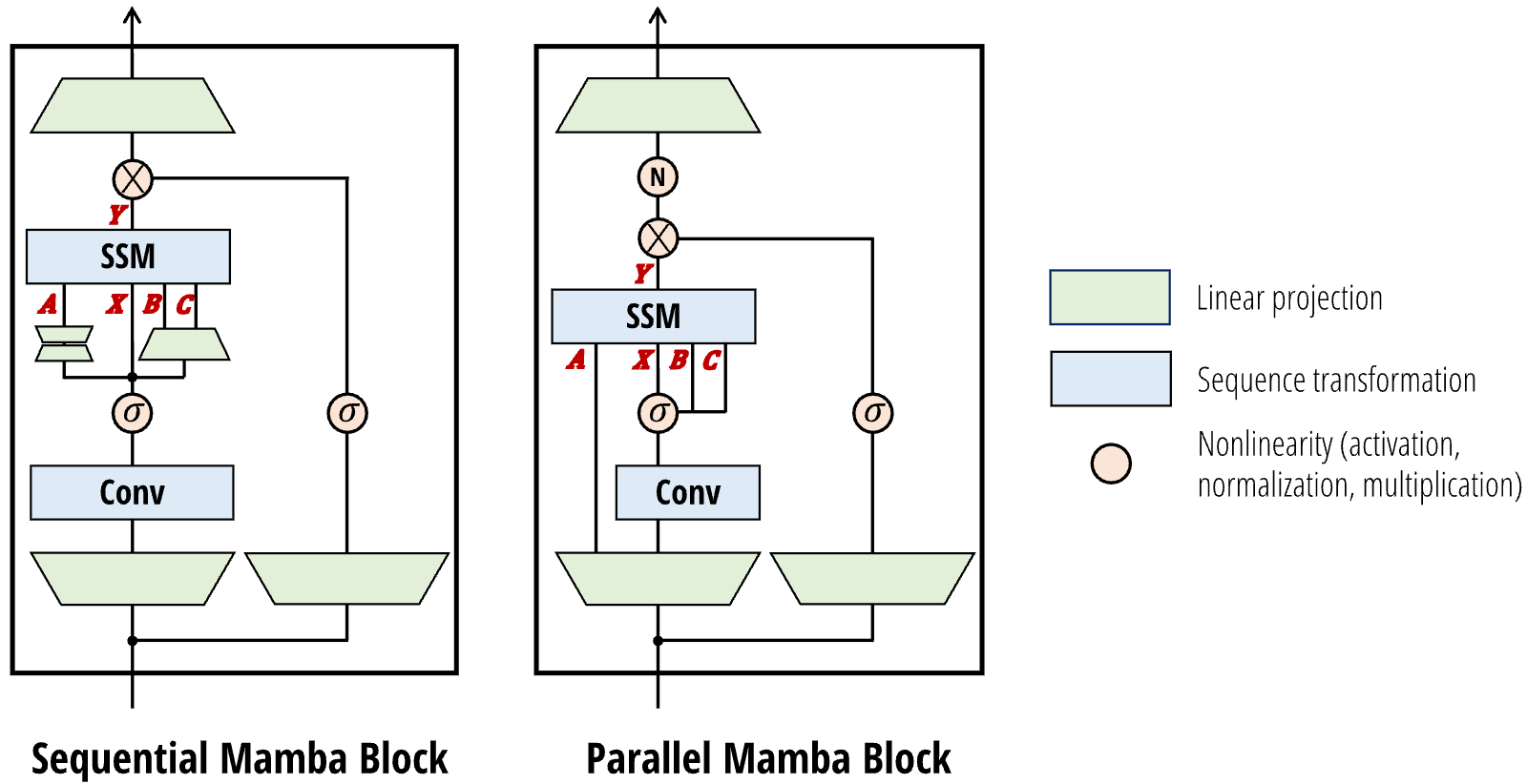
Figure 6: (**Mamba-2 Architecture**.) The Mamba-2 block simplifies the Mamba block by removing sequential linear projections; the SSM parameters $A,B,C$ are produced at the beginning of the block instead of as a function of the SSM input $X$ . An additional normalization layer is added as in NormFormer (Shleifer et al., 2021), improving stability. The $B$ and $C$ projections only have a single head shared across the $X$ heads, analogous to multi-value attention (MVA).

We first discuss modifications to the neural network block that are independent of the inner sequence mixing layer (i.e. outside the core SSD layer).

Mamba-1 was motivated by an SSM-centric point of view where the selective SSM layer is viewed as a map from $X\mapsto Y$ . The SSM parameters $A,B,C$ are viewed as subsidiary and are functions of the SSM input $X$ . Thus the linear projections defining $(A,B,C)$ occur after the initial linear projection to create $X$ .

In Mamba-2, the SSD layer is viewed as a map from $A,X,B,C\mapsto Y$ . It therefore makes sense to produce $A,X,B,C$ in parallel with a single projection at the beginning of the block. Note the analogy to standard attention architectures, where $X,B,C$ correspond to the $Q,K,V$ projections that are created in parallel.

Note that adopting parallel projections for the $A,B,C,X$ inputs to the SSM slightly reduces parameters and more importantly is more amenable to tensor parallelism for larger models, by using standard Megatron sharding patterns (Shoeybi et al., 2019)).

In preliminary experiments, we found that instabilities were prone to arising in larger models. We were able to alleviate this by adding an extra normalization layer (e.g. LayerNorm, GroupNorm, or RMSNorm) to the block right before the final output projection. This usage of a normalization is most directly related to the NormFormer architecture (Shleifer et al., 2021), which also added normalization layers at the end of the MLP and MHA blocks.

We also note that this change is similar to other recent models related to Mamba-2 that were derived from a linear attention viewpoint. The original linear attention formulation normalizes by a denominator term that emulates the normalization of the softmax function in standard attention. TransNormerLLM (Qin et al., 2023a) and RetNet (Sun et al., 2023) find that this normalization is unstable and add an extra LayerNorm or GroupNorm after the linear attention layer. Our extra normalization layer differs slightly from these, occuring after the multiplicative gate branch instead of before.

Recall that SSMs are defined as a sequence transformation (Definition 2.1) where:

•
$A,B,C$ parameters have a state dimension $\mathtt{N}$ .
•
They define a sequence transformation $\mathbb{R}^{\mathtt{T}}\to\mathbb{R}^{\mathtt{T}}$ , which for example can be represented as a matrix $M\in\mathbb{R}^{\mathtt{(T,T)}}$ .
•
This transformation operates over an input sequence $X\in\mathbb{R}^{\mathtt{(T,P)}}$ , independently over the $\mathtt{P}$ axis.

One can view this as defining one head of the sequence transformation.

Definition 7.1 (Multihead patterns).

A multihead sequence transformation consists of $\mathtt{H}$ independent heads, for a total model dimension of $\mathtt{D}=\mathtt{d\_model}$ . The parameters may be tied across heads, leading to a head pattern.

The state size $\mathtt{N}$ and head dimension $\mathtt{P}$ are analogous to the $QK$ head dimension and $V$ head dimension of attention, respectively. Just as in modern Transformer architectures (Chowdhery et al., 2023; Touvron et al., 2023), in Mamba-2 we generally choose these to be constants around $64$ or $128$ ; when the model dimension $\mathtt{D}$ increases, we increase the number of heads while keeping the head dimensions $\mathtt{N}$ and $\mathtt{P}$ fixed. In order to describe how to do this, we can transfer and generalize ideas from multihead attention to define similar patterns for SSMs, or any general sequence transformation.

\begin{aligned} & \displaystyle\textbf{Multi-head SSM} \\ & \displaystyle(\textrm{Multi-head Attn.}) \\ \displaystyle X & \displaystyle\mathtt{(T,H,P)} \\ \displaystyle A & \displaystyle\mathtt{(T,H)} \\ \displaystyle B & \displaystyle\mathtt{(T,H,N)} \\ \displaystyle C & \displaystyle\mathtt{(T,H,N)}\end{aligned}

\begin{aligned} & \displaystyle\textbf{Multi-contract SSM} \\ & \displaystyle(\textrm{Multi-query Attn.}) \\ \displaystyle X & \displaystyle\mathtt{(T,1,P)} \\ \displaystyle A & \displaystyle\mathtt{(T,H)} \\ \displaystyle B & \displaystyle\mathtt{(T,1,N)} \\ \displaystyle C & \displaystyle\mathtt{(T,H,N)}\end{aligned}

\begin{aligned} & \displaystyle\textbf{Multi-expand SSM} \\ & \displaystyle(\textrm{Multi-key Attn.}) \\ \displaystyle X & \displaystyle\mathtt{(T,1,P)} \\ \displaystyle A & \displaystyle\mathtt{(T,H)} \\ \displaystyle B & \displaystyle\mathtt{(T,H,N)} \\ \displaystyle C & \displaystyle\mathtt{(T,1,N)}\end{aligned}

\begin{aligned} & \displaystyle\textbf{Multi-input SSM} \\ & \displaystyle(\textrm{Multi-value Attn.}) \\ \displaystyle X & \displaystyle\mathtt{(T,H,P)} \\ \displaystyle A & \displaystyle\mathtt{(T,H)} \\ \displaystyle B & \displaystyle\mathtt{(T,1,N)} \\ \displaystyle C & \displaystyle\mathtt{(T,1,N)}\end{aligned}

The classic MHA pattern assumes that the head dimension $\mathtt{P}$ divides the model dimension $\mathtt{D}$ . The number of heads is defined as $\mathtt{H}=\mathtt{D}/\mathtt{P}$ . Then, $\mathtt{H}$ copies of the core sequence transformation are created by creating $\mathtt{H}$ independent copies of each parameter. Note that while the MHA pattern was first described for the attention sequence transformation, it can be applied to anything compatible with Definition 2.1. For example, a multi-head SSD layer would accept inputs with shapes according to equation (17) where the SSD algorithm is broadcasted over the $\mathtt{H}=\mathtt{n\_heads}$ dimension.

Multi-query attention (Shazeer, 2019) is a clever optimization for attention that can dramatically improve the speed of autoregressive inference, which relies on caching the $K$ and $V$ tensors. This technique simply avoids giving $K$ and $V$ the extra head dimension, or in other words broadcasts a single head of $(K,V)$ across all the heads of $Q$ .

Using the state space duality, we can define an equivalent SSM version of MQA as equation (18). Here, $X$ and $B$ (the SSM analogs of attention’s $V$ and $K$ ) are shared across the $\mathtt{H}$ heads. We also call this the multi-contract SSM (MCS) head pattern, because the $C$ parameter which controls the SSM state contraction has independent copies per head.

We can similarly define a multi-key attention (MKA) or multi-expand SSM (MES) head pattern, where $B$ (which controls the SSM expansion) is independent per head while $C$ and $X$ are shared across heads.

While MQA makes sense for attention because of its KV cache, it is not the natural choice for SSMs. In Mamba, instead, $X$ is viewed as the main input to the SSM, and therefore $B$ and $C$ are parameters that are shared across the input channels. We define a new multi-value attention (MVA) of multi-input SSM (MIS) pattern in equation (20), which can again be applied to any sequence transformation such as SSD.

Armed with this vocabulary, we can characterize the original Mamba architecture more precisely.

Proposition 7.2.

The selective SSM (S6) layer of the Mamba architecture (Gu & Dao, 2023) can be viewed as having

•
Head dimension $P=1$ : every channel has independent SSM dynamics $A$ .
•
Multi-input SSM (MIS) or multi-value attention (MVA) head structure: the $B,C$ matrices (corresponding to $K,Q$ in the attention duality) are shared across all channels of the input $X$ (corresponding to $V$ in attention).

We can also ablate these head pattern variants when applied to SSD (Section 9.4.3). Interestingly, despite being controlled in parameter counts and total state dimension, there is a noticeable difference in downstream performance. We empirically find that the MVA pattern as originally used in Mamba performs best.

The ideas of multi-query attention can be extended to grouped-query attention (Ainslie et al., 2023): instead of $1$ K and V head, one can create $\mathtt{G}$ independent K and V heads, where $1<\mathtt{G}$ and $\mathtt{G}$ divides $\mathtt{H}$ . This is motivated both by bridging the performance difference between multi-query and multi-head attention, and enabling more efficient tensor parallelism by setting $\mathtt{G}$ to be a multiple of the number of shards (Section 8).

Similarly, the multi-input SSM head pattern used in Mamba-2 can be easily extended to grouped-input SSM (GIS), or synonymously grouped-value attention (GVA). The generalization is straightforward and we omit the details for simplicity.

We describe here an example of architectural modifications to SSD motivated by linear attention. We ablate these in Section 9.4.3 as a form of negative result, finding that they do not significantly improve performance enough to adopt them as default settings. Nonetheless, these illustrate how the vast literature on attention can be incorporated to define variants of SSD. We treat the choice of kernel feature map as a hyperparameter in the Mamba-2 architecture, and expect other simple modifications inspired by attention to be possible as well.

Many variants of linear attention or kernel attention are motivated by viewing the attention scores $\mathsf{softmax}(QK^{\top})$ as composed of

1.
An exponential kernel $Z=\exp(QK^{\top})$ , which can be approximated by $Z=\psi(Q)\psi(K)^{\top}$ for some kernel feature map.
2.
Normalizing the kernel so that rows sum to $1$ via $M=G/G\bm{1}\bm{1}^{\top}$ , where the division happens elementwise and $\bm{1}$ is the all 1’s vector.

In Mamba-2, we incorporate a flexible kernel feature map, and apply it to the $B$ and $C$ branches (corresponding to the $K$ and $V$ branches in attention). The feature map can also be optionally applied to the $X$ ( $V$ ) branch, for simplicity and symmetry. This is represented in Figure 6 by an arbitrary nonlinearity. By default, we simply choose $\psi$ to be an elementwise Swish / SiLU function (Hendrycks & Gimpel, 2016; Ramachandran et al., 2017). We explore other options in the ablations in Section 9.4.3, including feature maps used by Linear Attention, Performer, Random Feature Attention, and cosFormer (Section 4.1.3).

To find the denominator term, we simply have to compute $M\bm{1}$ . But recall that the final output of the model is just $Y=MX$ (equation (16)). So the normalization terms can be found simply by augmenting $X$ with an extra column $\bm{1}$ , resulting in a tensor of shape $\mathtt{(T,P+1)}$ .

Note that in this case, the kernel feature map $\psi$ must be positive so that the sum is positive.

We describe several systems optimizations for SSMs, in particular the Mamba-2 architecture, for large-scale efficient training and inference. In particular, we focus on tensor parallel and sequence parallel for large-scale training, as a well variable-length sequences for efficient finetuning and inference.

Tensor parallelism (TP) (Shoeybi et al., 2019) is a model parallelism technique that splits each layer (e.g., attention, MLP) to run on multiple accelerators such as GPUs. This technique is widely used to train most large models (Brown et al., 2020; Chowdhery et al., 2023; Touvron et al., 2023; Touvron et al., 2023a) on GPU clusters where each node typically has 4-8 GPUs with fast networking such as NVLink. TP was originally developed for the Transformer architecture, and it is not straight-forward to adapt it other architecture. We first show the challenge of using TP with the Mamba architecture, and the show how the Mamba-2 architecture is designed to make TP efficient.

Recall the Mamba architecture, with a single input $u\in\mathbb{R}^{L\times d}$ (no batching for simplicity), input projection matrices $W^{(x)},W^{(z)}\in\mathbb{R}^{d\times ed}$ where $e$ is the expansion factor (typically 2), and output projection matrix $W^{(o)}\in\mathbb{R}^{ed\times d}$ :

\begin{aligned}\displaystyle x & \displaystyle=u{W^{(x)}}^{\top}\in\mathbb{R}^{L\times ed}\end{aligned}

\begin{aligned}\displaystyle z & \displaystyle=u{W^{(z)}}^{\top}\in\mathbb{R}^{L\times ed}\end{aligned}

\begin{aligned}\displaystyle x_{c} & \displaystyle=\mathrm{conv1d}(x)\in\mathbb{R}^{L\times ed}\quad\text{(depthwise, independent along $d$)}\end{aligned}

\begin{aligned}\displaystyle\Delta,B,C & \displaystyle=\text{low-rank projection}(x_{c})\end{aligned}

\begin{aligned}\displaystyle y & \displaystyle=SSM_{A,B,C,\Delta}(x_{c})\in\mathbb{R}^{L\times ed}\quad\text{(independent along $d$)}\end{aligned}

\begin{aligned}\displaystyle y_{g} & \displaystyle=y\cdot\phi(z)\quad\text{(gating, e.g., with $\phi$ being SiLU)}\end{aligned}

\begin{aligned}\displaystyle\mathrm{out} & \displaystyle=y_{g}{W^{(o)}}^{\top}\in\mathbb{R}^{L\times d}.\end{aligned}

With TP, suppose that we want to split the computation along 2 GPUs. It is easy to split the input projection matrices $W^{(x)}$ and $W^{(z)}$ into two partitions each of size $d\times\frac{ed}{2}$ . Then each GPU would hold half of $x_{c}$ of size $L\times\frac{ed}{2}$ . However, we see that since $\Delta,B,C$ are functions are $x_{c}$ , so we would need an extra all-reduce between the GPUs to get the whole of $x_{c}$ before computing $\Delta,B,C$ . After that the two GPUs can compute the SSM in parallel since they are independent along $d$ . At the end, we can split the output projection matrices $W^{(o)}$ into two partitions each of size $\frac{ed}{2}\times d$ , and do an all-reduce at the end. Compared to Transformers, we would incur two all-reduces instead of one, doubling the time spent in communication. For large-scale Transformers training, communication might already take a significant fraction of time (e.g. 10-20%), and doubling communication would make Mamba not as efficient for large-scale training.

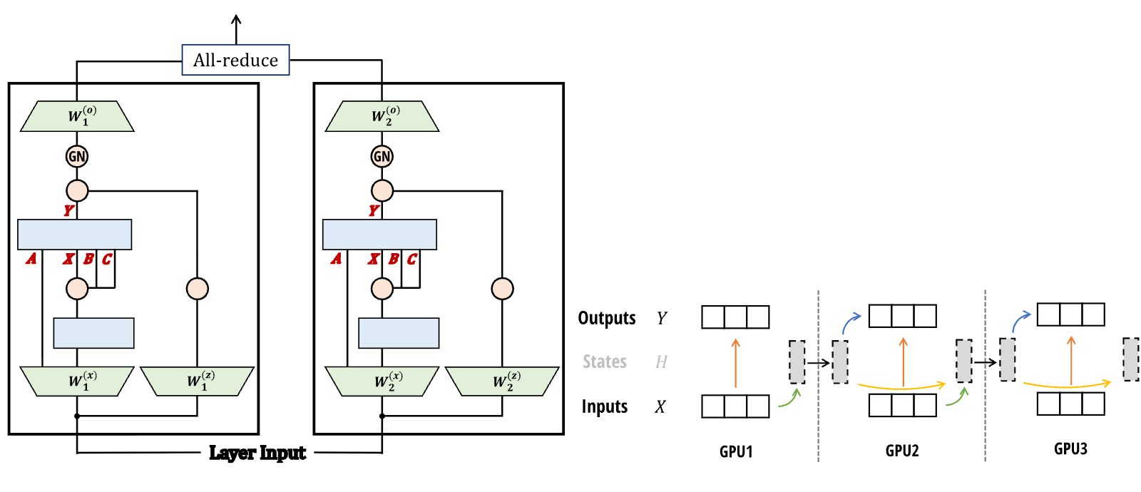
With Mamba-2, our goal is to have only one all-reduce per block, similar to attention or MLP blocks in Transformers. As a result, we have the projection to get $\Delta,B,C$ directly from $u$ instead of from $x_{c}$ , allowing us to split these projection matrices. This implies that we have different sets of $\Delta,B,C$ on different GPUs, which is equivalent to having several “groups” of $\Delta,B,C$ on a larger “logical GPU”. Moreover, we use GroupNorm within each block, with number of groups divisible by the TP degree, so that the GPUs in a TP group do not have a communicate within the block:

\begin{aligned}\displaystyle x & \displaystyle=u{W^{(x)}}^{\top}\in\mathbb{R}^{L\times ed}\end{aligned}

\begin{aligned}\displaystyle z & \displaystyle=u{W^{(z)}}^{\top}\in\mathbb{R}^{L\times ed}\end{aligned}

\begin{aligned}\displaystyle\Delta,B,C & \displaystyle=\text{projection}(u)\quad\text{(one or more groups of $\Delta,B,C$ per GPU)}\end{aligned}

\begin{aligned}\displaystyle x_{c} & \displaystyle=\mathrm{conv1d}(x)\in\mathbb{R}^{L\times ed}\quad\text{(depthwise, independent along $d$)}\end{aligned}

\begin{aligned}\displaystyle y & \displaystyle=SSM_{A,B,C,\Delta}(x_{c})\in\mathbb{R}^{L\times ed}\quad\text{(independent along $d$)}\end{aligned}

\begin{aligned}\displaystyle y_{g} & \displaystyle=y\cdot\phi(z)\quad\text{(gating, e.g., with $\phi$ being SiLU)}\end{aligned}

\begin{aligned}\displaystyle y_{n} & \displaystyle=\mathrm{groupnorm}(y_{g})\quad\text{(number of groups divisible by degree of tensor parallel)}\end{aligned}

\begin{aligned}\displaystyle\mathrm{out} & \displaystyle=y_{g}{W^{(o)}}^{\top}\in\mathbb{R}^{L\times d}.\end{aligned}

We see that we only need to split the input projection matrices, and the output projection matrices, and only need to do all-reduce at the end of the block. This is similar to the design of TP for attention and MLP layers. In particular, if we have TP degree 2, we would split $W^{(x)}=[W^{(x)}_{1},W^{(x)}_{2}]$ with $W^{(x)}_{i}\in\mathbb{R}^{d\times ed/2}$ , $W^{(z)}=[W^{(z)}_{1},W^{(z)}_{2}]$ with $W^{(z)}_{i}\in\mathbb{R}^{d\times ed/2}$ , and $W^{(o)}=\begin{bmatrix}W^{(o)}_{1}\\ W^{(o)}_{2}\end{bmatrix}$ with $W^{(o)}_{i}\in\mathbb{R}^{ed/2\times d}$ . For $i=1,2$ , the TP Mamba-2 layer can be written as:

\begin{aligned}\displaystyle x^{(i)} & \displaystyle=u{W^{(x)}_{i}}^{\top}\in\mathbb{R}^{L\times ed/2}\end{aligned}

\begin{aligned}\displaystyle z^{(i)} & \displaystyle=u{W^{(z)}_{i}}^{\top}\in\mathbb{R}^{L\times ed/2}\end{aligned}

\begin{aligned}\displaystyle\Delta^{(i)},B^{(i)},C^{(i)} & \displaystyle=\text{projection}(u)\quad\text{(one or more groups of $\Delta,B,C$ per GPU)}\end{aligned}

\begin{aligned}\displaystyle x_{c}^{(i)} & \displaystyle=\mathrm{conv1d}(x^{(i)})\in\mathbb{R}^{L\times ed/2}\end{aligned}

\begin{aligned}\displaystyle y^{(i)} & \displaystyle=SSM_{A,B,C,\Delta}(x_{c}^{(i)})\in\mathbb{R}^{L\times ed/2}\end{aligned}

\begin{aligned}\displaystyle y_{g}^{(i)} & \displaystyle=y^{(i)}\cdot\phi(z^{(i)})\end{aligned}

\begin{aligned}\displaystyle y_{n}^{(i)} & \displaystyle=\mathrm{groupnorm}(y_{g}^{(i)})\quad\text{(number of groups divisible by degree of tensor parallel)}\end{aligned}

\begin{aligned}\displaystyle\mathrm{out}^{(i)} & \displaystyle=y_{g}^{(i)}{W^{(o)}_{i}}^{\top}\in\mathbb{R}^{L\times d/2}\end{aligned}

\begin{aligned}\displaystyle\mathrm{out} & \displaystyle=\sum_{i}\mathrm{out}^{(i)}.\quad\text{(summing outputs from all GPUs with an all-reduce)}\end{aligned}

We illustrate tensor parallel with Mamba-2 in Figure 7 (Left).

Figure 7: (**Parallelism with the Mamba-2 Block**.) (Left: **Tensor Parallelism**) We split the input projection matrices $W^{(x)},W^{(z)}$ and the output projection matrix $W^{(o)}$ . Each SSM head $(A,B,C,X)\mapsto Y$ lives on a single device. Choosing GroupNorm for the final normalization layer avoids extra communication. We need one all-reduce per layer, just like the MLP or attention blocks in a Transformer. (Right: **Sequence/Context Parallelism**) Analogous to the SSD algorithm, with multiple devices, we can split along the sequence dimension. Each device computes the state of its sequence, then pass that state to the next GPU.

For very long sequences, we might need to split the input and activation to different GPUs along the sequence length dimension. There are two main techniques:

1.
Sequence parallelism (SP) for the residual and normalization operations: first proposed by Korthikanti et al. (2023), this technique decomposes the all-reduce in TP as reduce-scatter and all-gather. Noticing that the residual and normalization operations are repeated on the same input for all GPUs in the same TP group, SP splits the activations along the sequence length dimension by performing: reduce-scatter, residual and normalization, then all-gather.
Since the Mamba-2 architecture uses the same residual and normalization structure, SP applies without modification.
2.
Sequence parallelism for the token-mixing operations (attention or SSM), also known as “context parallelism” (CP). Several techniques have been developed for attention layer (e.g., Ring attention (Liu et al., 2023; Liu et al., 2024)), with sophisticated load-balancing technique (Brandon et al., 2023). The difficulty with sequence parallelism in attention is that we can split queries and keys into block, but each query block needs to interact with key blocks, leading to communication bandwidth quadratic in the number of workers.
With SSMs, we can split the sequence in a simple manner: each worker takes an initial state, compute the SSM with respect to their inputs, return the final state, and pass that final state to the next worker. The communication bandwidth is linear in the number of workers. This decomposition is exactly the same as the block-decomposition in the SSD algorithm (Figure 5) to split into blocks / chunks. We illustrate this context parallelism in Figure 7 (Right).

While pretraining often uses the same sequence lengths for the batch, during finetuning or inference, the model might need to process different input sequences of different lengths. One naive way to handle this case is to right-pad all sequences in the batch to the maximum length, but this can be inefficient if sequences are wildly different lengths. For transformers, sophisticated techniques have been develop to avoid padding and do load-balancing between GPUs (Zeng et al., 2022; Zhai et al., 2023), or packing multiple sequences in the same batch and adjust the attention mask (Ding et al., 2024; Pouransari et al., 2024). With SSMs and Mamba in particular, we can handle variable sequence lengths by simply treating the whole batch as one long sequence, and avoid passing the states between individual sequences. This is equivalent to simply setting $A_{t}=0$ for tokens $t$ at the end of one sequence to prevent it from passing information to the token $t+1$ , which belongs to a different sequence.

We empirically evaluate Mamba-2 on synthetic recall tasks that have been challenging for recurrent models (Section 9.1), and standard language modeling pre-training and downstream evaluations (Section 9.2). We validate that our SSD algorithm is much more efficient than Mamba-1 (Section 9.3) and comparable to optimized attention for moderate sequence lengths. Finally, we ablate various design choices in the Mamba-2 architecture (Section 9.4).

Figure 8: (**Multi-Query Associative Recall (MQAR)**). Associative recall tasks are challenging for SSMs, which must memorize all relevant information into their recurrent state. The SSD layer combined with improved architecture allows for much larger state sizes in Mamba-2, which performs significantly better than Mamba-1 and even vanilla attention.

Figure 9: (**Scaling Laws**.) Models of size $\approx 125M$ to $\approx 1.3B$ parameters, trained on the Pile. Mamba-2 matches or exceeds the performance of Mamba as well as a strong “Transformer++” recipe. Compared to our Transformer baseline, Mamba-2 is Pareto dominant on performance (perplexity), theoretical FLOPs, and actual wall-clock time.

Original Table 1 — Table 1: (**Zero-shot Evaluations**.) Best results for each size in bold, second best unlined. We compare against open source LMs with various tokenizers, trained for up to 300B tokens. Pile refers to the validation split, comparing only against models trained on the same dataset and tokenizer (GPT-NeoX-20B). For each model size, Mamba-2 outperforms Mamba, and generally matches Pythia at twice the model size. Full results in Table 8.

Table 1
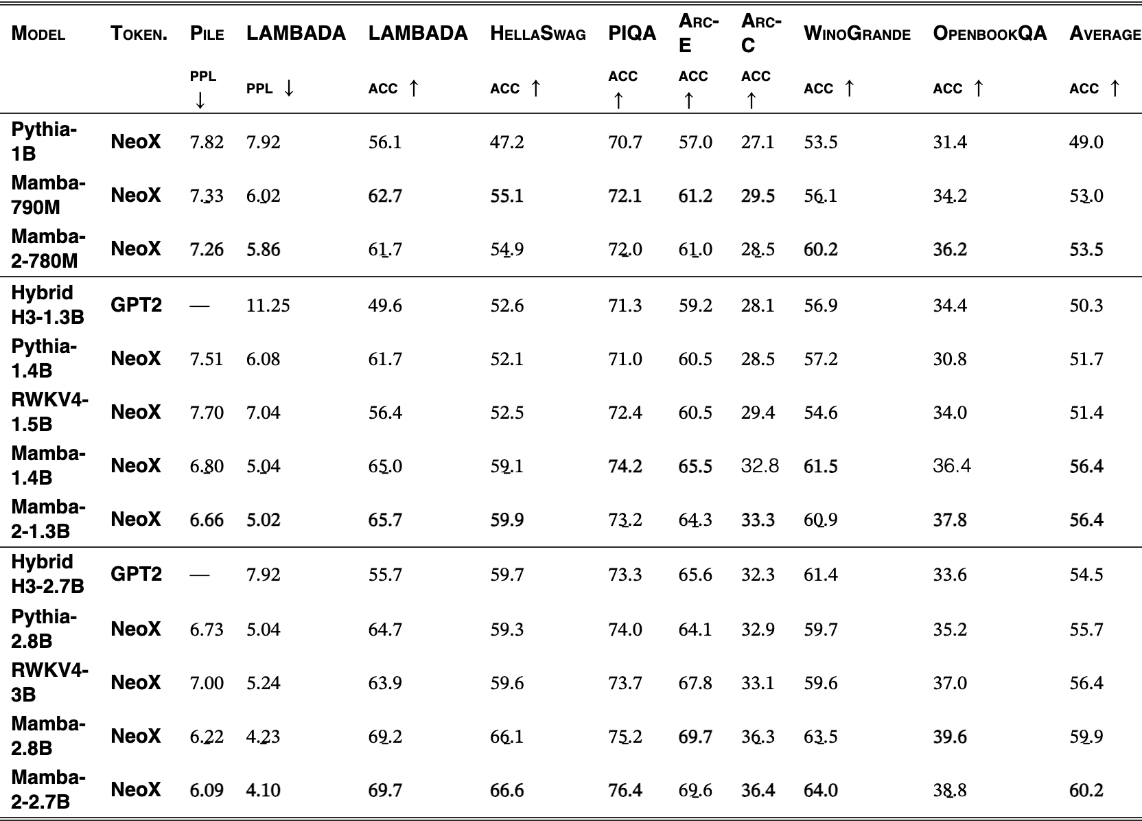
Model	Token.	Pile	LAMBADA	LAMBADA	HellaSwag	PIQA	Arc-E	Arc-C	WinoGrande	OpenbookQA	Average
Pythia-1B	NeoX	$7.82$	$7.92$	$56.1$	$47.2$	$70.7$	$57.0$	$27.1$	$53.5$	$31.4$	$49.0$
Mamba-790M	NeoX	$\underline{7.33}$	$\underline{6.02}$	$\mathbf{62.7}$	$\mathbf{55.1}$	$\mathbf{72.1}$	$\mathbf{61.2}$	$\mathbf{29.5}$	$\underline{56.1}$	$\underline{34.2}$	$\underline{53.0}$
Mamba-2-780M	NeoX	$\mathbf{7.26}$	$\mathbf{5.86}$	$\underline{61.7}$	$\underline{54.9}$	$\underline{72.0}$	$\underline{61.0}$	$\underline{28.5}$	$\mathbf{60.2}$	$\mathbf{36.2}$	$\mathbf{53.5}$
Hybrid H3-1.3B	GPT2	—	$11.25$	$49.6$	$52.6$	$71.3$	$59.2$	$28.1$	$56.9$	$34.4$	$50.3$
Pythia-1.4B	NeoX	$7.51$	$6.08$	$61.7$	$52.1$	$71.0$	$60.5$	$28.5$	$57.2$	$30.8$	$51.7$
RWKV4-1.5B	NeoX	$7.70$	$7.04$	$56.4$	$52.5$	$72.4$	$60.5$	$29.4$	$54.6$	$34.0$	$51.4$
Mamba-1.4B	NeoX	$\underline{6.80}$	$\underline{5.04}$	$\underline{65.0}$	$\underline{59.1}$	$\mathbf{74.2}$	$\mathbf{65.5}$	32.8	$\mathbf{61.5}$	36.4	$\mathbf{56.4}$
Mamba-2-1.3B	NeoX	$\mathbf{6.66}$	$\mathbf{5.02}$	$\mathbf{65.7}$	$\mathbf{59.9}$	$\underline{73.2}$	$\underline{64.3}$	$\mathbf{33.3}$	$\underline{60.9}$	$\mathbf{37.8}$	$\mathbf{56.4}$
Hybrid H3-2.7B	GPT2	—	$7.92$	$55.7$	$59.7$	$73.3$	$65.6$	$32.3$	$61.4$	$33.6$	$54.5$
Pythia-2.8B	NeoX	$6.73$	$5.04$	$64.7$	$59.3$	$74.0$	$64.1$	$32.9$	$59.7$	$35.2$	$55.7$
RWKV4-3B	NeoX	$7.00$	$5.24$	$63.9$	$59.6$	$73.7$	$67.8$	$33.1$	$59.6$	$37.0$	$56.4$
Mamba-2.8B	NeoX	$\underline{6.22}$	$\underline{4.23}$	$\underline{69.2}$	$\underline{66.1}$	$\underline{75.2}$	$\mathbf{69.7}$	$\underline{36.3}$	$\underline{63.5}$	$\mathbf{39.6}$	$\underline{59.9}$
Mamba-2-2.7B	NeoX	$\mathbf{6.09}$	$\mathbf{4.10}$	$\mathbf{69.7}$	$\mathbf{66.6}$	$\mathbf{76.4}$	$\underline{69.6}$	$\mathbf{36.4}$	$\mathbf{64.0}$	$\underline{38.8}$	$\mathbf{60.2}$

Figure 10: (**Efficiency Benchmarks**.) (Left) Our SSD is $2-8\times$ faster than a Mamba fused scan for large state expansion ( $N=64$ ) and faster than FlashAttention-2 for sequence length 2k and above. (Right) Sequence length 4K: Increasing state expansion slows down the Mamba optimized scan implementation linearly. SSD can handle much larger state expansion factors without much slowdown.

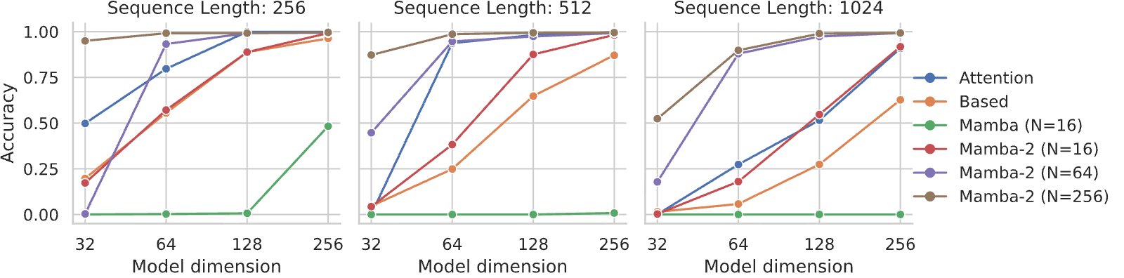
Synthetic associative recall tasks have been popular for testing the ability of language models to look up information in their context. Broadly, they involve feeding autoregressive models pairs of key-value associations, and then prompting the model to produce the correct completion upon being shown a previously-seen key. The multi-query associative recall (MQAR) task is a particular formulation of this task that requires the model to memorize multiple associations (Arora et al., 2024). The original Mamba paper reported results on related synthetic tasks, in particular Selective Copying (Gu & Dao, 2023) and Induction Heads (Olsson et al., 2022), which can be seen as easier associative recall tasks. The MQAR task is also closely related to “phonebook look-up” tasks which has been shown to be challenging for recurrent models such as SSMs, due to their finite state capacity (Jelassi et al., 2024; De et al., 2024).

We compare on a challenging version of the MQAR setup from (Arora et al., 2024a), using a harder task, longer sequences, and smaller models. Our baselines include standard multi-head softmax attention as well as the Based architecture which combines convolutions, local attention, and a linear attention variant.

Results are shown in Figure 8. While Mamba-1 struggles on this task, Mamba-2 performs well across all settings. Surprisingly, it is significantly better than Mamba-1 even when the state sizes are controlled ( $\mathtt{N}=16$ ). (We are not sure which aspect of the architecture is the predominant factor, which remains a question to explore in future work.) Additionally, this task validates the importance of state size: increasing from $\mathtt{N}=16$ to $\mathtt{N}=64$ and $\mathtt{N}=256$ consistently improves performance on MQAR, as the larger state allows more information (key-value pairs) to be memorized.

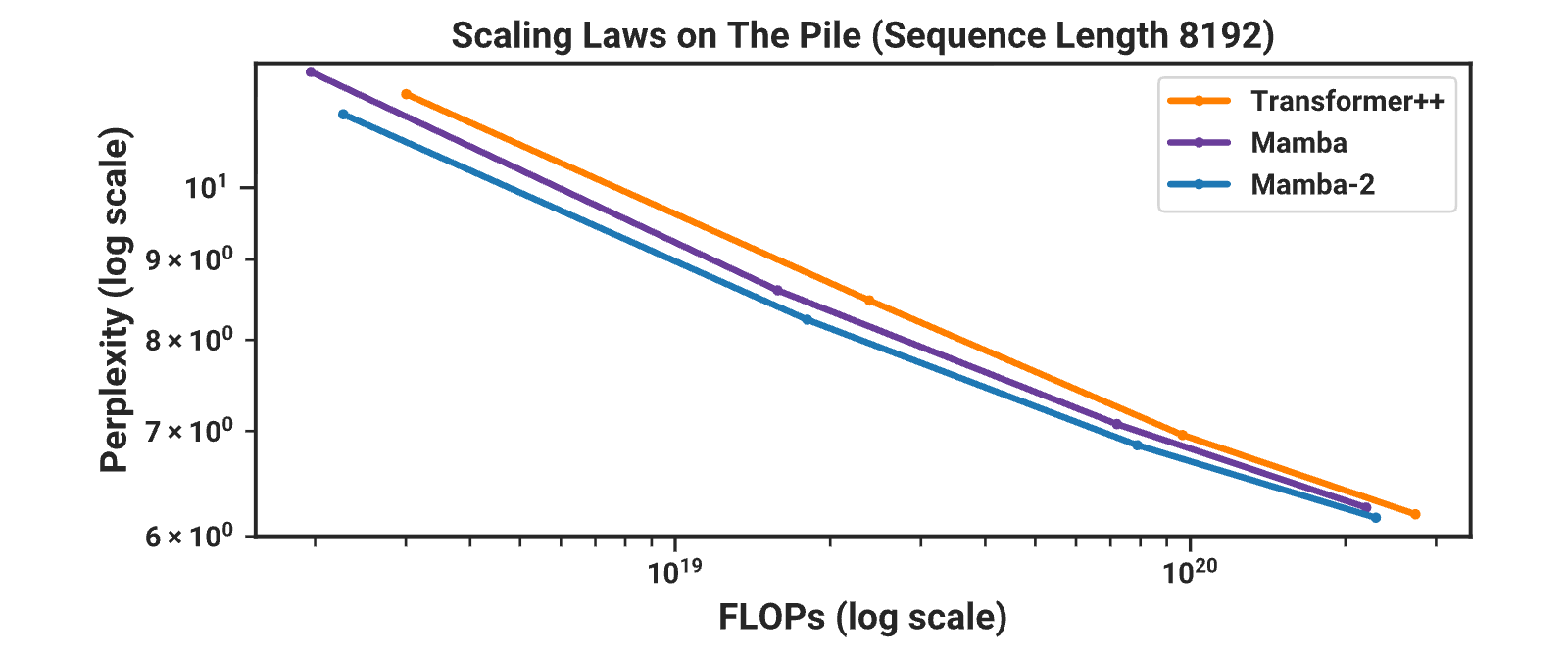
Following standard protocols in LLMs, we train and evaluate the Mamba-2 architecture on standard autoregressive language modeling against other architectures. We compare both pretraining metrics (perplexity) and zero-shot evaluations. The model sizes (depth and width) follow GPT3 specifications, from 125m to 2.7B. We use the Pile dataset (Gao et al., 2020), and follow the training recipe described in Brown et al. (2020). This follows the same setup as reported in Mamba (Gu & Dao, 2023); training details are in Appendix D.

For baselines, we compare against both Mamba and its Transformer++ recipe (Gu & Dao, 2023), which is based on the PaLM and LLaMa architectures (e.g. rotary embedding, SwiGLU MLP, RMSNorm instead of LayerNorm, no linear bias, and higher learning rates). As Mamba has already demonstrated that it outperforms the standard Transformer architecture (GPT3 architecture) as well as recent subquadratic architectures (H3 (Dao et al., 2023), Hyena (Poli et al., 2023), RWKV-4 (Peng et al., 2023), RetNet (Sun et al., 2023)), we omit those in the plot for clarity (see Gu & Dao (2023) for comparisons).

Figure 9 shows scaling laws under the standard Chinchilla (Hoffmann et al., 2022) protocol, on models from $\approx 125M$ to $\approx 1.3B$ parameters.

Table 1 shows the performance of Mamba-2 on a range of popular downstream zero-shot evaluation tasks, compared to the most well-known open source models at these sizes, most importantly Pythia (Biderman et al., 2023) which were trained with the same tokenizer, dataset, and training length (300B tokens) as our models.

Recent and concurrent work (Dao et al., 2023; De et al., 2024; Lieber et al., 2024; Glorioso et al., 2024) suggests that a hybrid architecture with both SSM layers and attention layers could improve the model quality over that of a Transformer, or a pure SSM (e.g., Mamba) model, especially for in-context learning. We explore the different ways that SSD layers can be combined with attention and MLP to understand the benefits of each. Empirically we find that having around 10% of the total number of layers being attention performs best. Combining SSD layers, attention layers, and MLP also works better than either pure Transformer++ or Mamba-2.

We find that SSD and attention layers are complementary: by themselves (e.g. in the Mamba-2 architecture vs. Transformer++) their performance (measured by perplexity) is nearly the same, but a mixture of SSD and attention layers outperforms the pure Mamba-2 or Transformer++ architecture. We show some results (Table 2) for the 350M model (48 layers) trained to 7B tokens on the Pile with the GPT-2 tokenizer (same number of parameters, same hyperparameters, same training and validation set). Adding in just a few attention layers already yields notable improvement and strikes the best balance between quality and efficiency. We hypothesize that the SSM layers function well as a general sequence-to-sequence mapping, and attention layers act as a retrieval mechanism to quickly refer to previous tokens in the sequence instead of forcing the model to compress all the context to its memory (SSM states).

Original Table 2 — Table 2: (**Combining SSD and Attention Blocks**.) Perplexity of a 350M model with 48 layers, with different number of attention layers. Having around a 10% ratio of attention layers performs best.

Table 2
Num. Attn Blocks	0 (Mamba-2)	1	2	3	4	5	6	7	9	11	15	24	Transformer++
Perplexity $\downarrow$	8.60	8.38	8.32	8.29	8.29	8.28	8.26	8.27	8.28	8.30	8.34	8.50	8.68

We compare different ways that SSD can be combined with the (gated) MLP and attention layers, and evaluate at the 2.7B scale (64 layers), trained to 300B tokens on the Pile (same number of parameters, same hyperparameters, same training and validation set, same data order):

1.
Transformer++: 32 attention layers and 32 gated MLP, interleaving.
2.
Mamba-2: 64 SSD layers.
3.
Mamba-2-MLP: 32 SSD and 32 gated MLP layers, interleaving.
4.
Mamba-2-Attention: 58 SSD layers and 6 attention layers (at indices 9, 18, 27, 36, 45, 56) $^{6}$ .
5.
Mamba-2-MLP-Attention: 28 SSD layers and 4 attention layers, interleaving with 32 gated MLP layers.

We report the validation perplexity on the Pile, as well as zero-shot evaluation, in Table 3. In general, the quality of Transformer++ and Mamba-2 models are around the same. We see that adding just 6 attention layers noticeably improves over the pure Mamba-2 model (and over Transformer++). Adding MLP layers reduces model quality, but can (i) speed up training and inference due to the simplicity and hardware-efficiency of the MLP layer (ii) be easier to up-cycle to MoE models by replacing MLP layers with mixture-of-experts.

Original Table 3 — Table 3: (**Zero-shot Evaluations**.) Best results for each size in bold. We compare different ways SSD, MLP, and attention layers can be combined, evaluated at 2.7B scale trained to 300B tokens on the Pile.

Table 3
Model	Token.	Pile	LAMBADA	LAMBADA	HellaSwag	PIQA	Arc-E	Arc-C	WinoGrande	OpenbookQA	Average
		ppl $\downarrow$	ppl $\downarrow$	acc $\uparrow$	acc $\uparrow$	acc $\uparrow$	acc $\uparrow$	acc $\uparrow$	acc $\uparrow$	acc $\uparrow$	acc $\uparrow$
Transformer++	NeoX	6.13	3.99	70.3	66.4	75.2	67.7	37.8	63.9	40.4	60.2
Mamba-2	NeoX	6.09	4.10	69.7	66.6	76.4	69.6	36.4	64.0	38.8	60.2
Mamba-2-MLP	NeoX	6.13	4.18	69.3	65.0	76.4	68.1	37.0	63.1	38.2	59.6
Mamba-2-Attention	NeoX	5.95	3.85	71.1	67.8	75.8	69.9	37.8	65.3	39.0	61.0
Mamba-2-MLP-Attention	NeoX	6.00	3.95	70.0	66.6	75.4	70.6	38.6	64.6	39.2	60.7

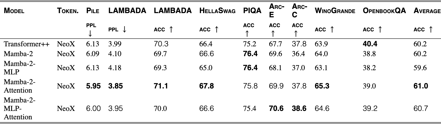
We benchmark the speed of the SSD algorithm against Mamba’s scan implementation and FlashAttention-2 (Figure 10). SSD, thanks to its reformulation to use matrix multiplication as a subroutine, can exploit specialized matrix multiplication (matmul) units on GPUs, also known as tensor cores. As a result, it is 2-8 $\times$ faster than Mamba’s fused associative scan, which does not leverage matmul units. Due to its linear scaling in sequence length, SSD is faster than FlashAttention-2 starting at sequence length $2K$ .

However, we note that the Mamba-2 model as a whole might not be as efficient to train as Transformer at short sequence length (e.g. at $2K$ ), since a Transformer with $L$ layers would have $\frac{L}{2}$ MLP layers and $\frac{L}{2}$ attention layers, while a Mamba-2 model would have $L$ SSD layers for the same number of parameters. Generally the MLP layers are very hardware efficient since they consist of simple matrix multiplication and pointwise linearity. As shown in Section 9.2.3, one can also combine $\frac{L}{2}$ SSD layers and $\frac{L}{2}$ MLP layers to speed up training at short sequence length.

Section 7.1 introduces the Mamba-2 block, which has small modifications to the Mamba-1 block which are partly motivated by the connection to attention and also to improve the scalability of Mamba-2. Table 4 ablates these architecture changes to the block, which occur outside of the core SSM layer.

The ablations validate that parallel projections to create $(A,B,C,X)$ saves parameters and performs slightly better than Mamba’s sequential projections. More importantly, this modification is amenable to tensor parallelism at larger model sizes (Section 8). Additionally, the extra normalization layer also slightly improves performance. More importantly, preliminary experiments at larger scales observed that it also helps with training stability.

Original Table 4 — Table 4: (**Ablations: Mamba-2 block**.) We ablate the major differences between the Mamba-2 and Mamba-1 neural network blocks (Figure 6, Section 7.1). Note that these components are independent of the inner sequence mixing layer; in these ablations, we use SSD for the inner SSM layer (differing from the S6 layer of Mamba-1).

Table 4
Block	$ABCX$ Projections	Extra Normalization	Parameters	Perplexity
Mamba-1	Sequential	✗	129.3M	11.76
	Sequential	✓	129.3M	11.54
	Parallel	✗	126.5M	11.66
Mamba-2	Parallel	✓	126.5M	11.49

Section 7.2 describes how the dimensions of the $B,C,X$ projections can be viewed as a hyperparameter analogous to notions of multi-head attention and multi-query attention. We also showed how the original Mamba architecture is analogous to multi-value attention (Proposition 7.2), which was a choice that naturally developed from the state-space model point of view and was not previously ablated.

Table 5 ablates choices of the multi-head structure for the Mamba-2 architecture. Strikingly, we find a large difference between multi-value and multi-query or multi-key head patterns, despite seeming very similar. Note that this is not explained by the total state size, which is the same for all of them (equal to $\mathtt{HPN}$ or the product of the number of heads, head dimension, and state dimension).

We also compare to multi-head patterns where the number of $C,B,X$ (analogous to $Q,K,V$ ) heads is equal. We compare against the standard multi-head pattern, as well as one with aggressive sharing where they all have only $1$ head. Note that in the latter case, the model still has $\mathtt{H}$ different sequence mixers $M$ , because each head still has a different $A$ . When parameter matched, these multi-head patterns perform similarly to each other, in between the MVA and MQA/MKA patterns.

Original Table 5 — Table 5: (**Ablations: Multi-head structure**.) All models have state expansion factor $N=64$ and head size $P=64$ and are trained to Chinchilla scaling law token counts. The number of $A$ heads is always equal to the total heads $\mathtt{H}$ , i.e. each head has a separate input-dependent $A$ decay factor. (Top) 125M models, 2.5B tokens (Bottom) 360M models, 7B tokens

Table 5
SSM Head Pattern	Attn. Analog	$A$ heads	$B$ heads	$C$ heads	$X$ heads	Layers	Params	Ppl.
Multi-input (MIS)	Multi-value (MVA)	24	1	1	24	24	126.5M	$\mathbf{11.66}$
Multi-contract (MCS)	Multi-query (MQA)	24	1	24	1	24	126.5M	$12.62$
Multi-expand (MES)	Multi-key (MKA)	24	24	1	1	24	126.5M	$12.59$
Multi-head (MHS)	Multi-head (MHA)	24	24	24	24	15	127.6M	$12.06$
Multi-state (MSS)	-	24	1	1	1	36	129.6M	$12.00$
Multi-input (MIS)	Multi-value (MVA)	32	1	1	32	48	361.8M	$\mathbf{8.73}$
Multi-contract (MCS)	Multi-query (MQA)	32	1	32	1	48	361.8M	$9.33$
Multi-expand (MES)	Multi-key (MKA)	32	32	1	1	48	361.8M	$9.36$
Multi-head (MHS)	Multi-head (MHA)	32	1	1	1	70	361.3M	$9.01$
Multi-state (MSS)	-	32	32	32	32	29	357.3M	$9.04$

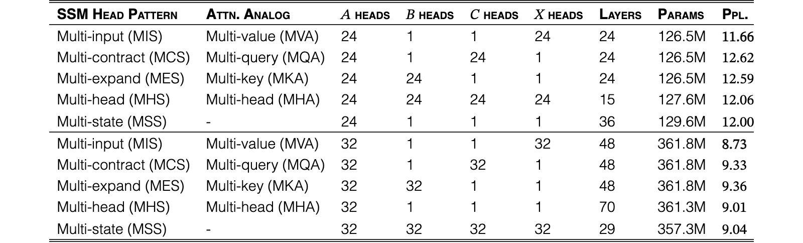
Section 7.3 noted how SSD can be combined with ideas from the linear attention literature, such as various forms of kernel approximations. We ablate several variants of these suggested by previous works in Figure 12. These include the cosFormer (Qin et al., 2022a), Random Feature Attention Peng et al., 2021, and Positive Random Features (Performer) (Choromanski et al., 2021).

We also ablate adding a normalization term, akin to the denominator of the softmax function in standard attention. We found that this introduced instabilities to most variants, but slightly improved performance for the ReLU activation function $\psi$ .

Figure 12 also tests more recent proposals to improve linear attention that involve expanding the feature dimension (Based (Arora et al., 2024a) and ReBased (Aksenov et al., 2024)). These linear attention extensions aim to appropriate the $\exp$ kernel with a quadratic approximation. ReBased also proposes to replace the QK activation function with a layer normalization; from an SSM-centric view we apply a normalization on top of $(B,C)$ before applying the SSM function. We note that this technique has been independently proposed as the “QK-Norm” for softmax attention (Team, 2024) and an “internal normalization” for Mamba (Lieber et al., 2024).

Overall, Figure 12 and Figure 12 found that the kernel approximation methods we tried did not seem to improve over simple pointwise non-linear activation functions for $\psi$ . Thus our default settings for Mamba-2 used $\psi(x)=\mathsf{Swish}(x)$ to follow Mamba-1, but we suggest that removing this activation entirely may be a simpler choice that we did not extensively test.

We emphasize however that SSD and vanilla linear attention differ in the inclusion of the 1-semiseparable mask $L$ , while the various linear attention methods in the literature were derived to approximate softmax attention without this term; thus, our negative results may be not unexpected.

Paper table
Kernel activation $\varphi$	Perplexity
none	$11.58$
Swish	$11.66$
Exp	$11.62$
ReLU	$11.73$
ReLU + normalization	$11.64$
cosFormer	$11.97$
Random Feature Attention	$11.57$
Positive Random Features (Performer)	$12.21$

Paper table
Kernel activation $\varphi$	Perplexity
Swish	$11.67$
Swish + Taylor (Based)	$12.19$
LayerNorm	$11.50$
LayerNorm + Square (ReBased)	$11.84$
Swish	$8.58$
Swish + Taylor (Based)	$8.71$
LayerNorm	$8.61$
LayerNorm + Square (ReBased)	$8.63$

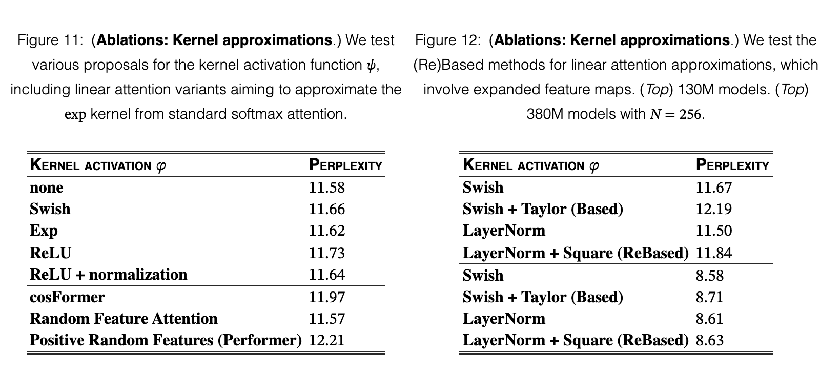
The state space duality framework bridges connections between SSMs, structured matrices, and attention. We discuss in more depth the relations between SSD and these concepts more broadly. Using ideas from each of the viewpoints, we also suggest some directions that the SSD framework can be extended in future work.

Structured state space models can be characterized along the axes

(i)
whether it is time-invariant or time-varying.
(ii)
the dimensionality of the system.
(iii)
the structure on the recurrent transitions $A$ .

SSD can be described as a selective SSM with SISO dimensions and scalar-identity structure.

The original structured SSMs (S4) were linear time-invariant (LTI) systems (Gu, 2023; Gu et al., 2022) motivated by continuous-time online memorization (Gu et al., 2020; Gu et al., 2021; Gu et al., 2023). Many variants of structured SSMs have been proposed (Gupta et al., 2022; Gu et al., 2022a; Smith et al., 2023; Ma et al., 2023; Dao et al., 2023), including several that drop the recurrence and focus on the convolutional representation of LTI SSMs (Li et al., 2023; Poli et al., 2023; Fu et al., 2023; Qin et al., 2023).

SSD is a time-varying structured SSM, also known as a selective SSM introduced in Mamba (Gu & Dao, 2023). Selective SSMs are closely related to gating mechanisms of RNNs, including classical RNNs such as the LSTM (Hochreiter & Schmidhuber, 1997) and GRU (Chung et al., 2014) as well as more modern variants such as the QRNN (Bradbury et al., 2016), SRU (Lei et al., 2017; Lei, 2021), RWKV (Peng et al., 2023), HGRN (Qin et al., 2023b), and Griffin (De et al., 2024; Botev et al., 2024). These RNNs differ in their parameterizations in various ways, most importantly in the lack of a state expansion.

An important characteristic of SSD, shared by previous SSMs in its lineage (S4, H3, Mamba), is that it is a single-input single-output (SISO) system where input channels are processed independently. This leads to a much larger effective state size of $\mathtt{ND}$ where $\mathtt{N}$ is the SSM state size (also called state expansion factor) and $\mathtt{D}$ is the standard model dimension. Traditional RNNs either have $\mathtt{N}=1$ or are multi-input multi-output (MIMO) with dense $B,C$ matrices, either of which leads to a smaller state. While MIMO SSMs have been shown to work well in some domains (Smith et al., 2023; Orvieto et al., 2023; Lu et al., 2023), Mamba showed that state expansion is crucial for information-dense domains such as language. One of the main advantages of SSD is allowing for even larger state expansion factors without slowing down the model. Many subsequent works have since adopted state expansion (Section 10.4).

Compared to previous structured SSMs, the main restriction of SSD is on the expressivity of the state transitions $A_{t}$ . We note that more general SSMs, such as the case of diagonal $A_{t}$ , have the same theoretical efficiency as SSD, but are less hardware-friendly. This is because the dual quadratic form loses its attention-like interpretation and becomes more difficult to compute. Thus compared to Mamba, SSD differs only in a slightly more restrictive form of diagonal $A_{t}$ , and trades off this expressivity for improved hardware efficiency (and ease of implementation).

We hypothesize that it may be possible to refine our structured matrix algorithms to improve to the general diagonal SSM case as well.

The first viewpoint of the state space duality adopts the viewpoint of these models as matrix sequence transformations or “matrix mixers”: sequence transformations (Definition 2.1) that can be represented as matrix multiplication (by a $\mathtt{T}\times\mathtt{T}$ matrix) along the sequence dimension $\mathtt{T}$ .

Several such matrix mixers have been proposed before, where the primary axis of variation is the representation of the matrix. These include MLP-Mixer (Tolstikhin et al., 2021) (unstructured matrix), FNet (Lee-Thorp et al., 2021) (Fourier Transform matrix), M2 (Dao et al., 2019; Dao et al., 2020; Dao et al., 2022; Fu et al., 2024) (butterfly/monarch matrix), Toeplitz matrices (Poli et al., 2023; Qin et al., 2023), and even more exotic structures (De et al., 2018; Thomas et al., 2018).

An important characterization is that efficient (sub-quadratic) matrix sequence transformations are exactly those which have structured matrix mixers. A core result of the SSD framework is viewing SSMs as matrix mixers with a particular structure – semiseparable matrices (Section 3). The linear vs. quadratic duality then takes the form of structured matrix multiplication vs. naive matrix multiplication.

The structure matrix representation led to our efficient SSD algorithm through block decompositions of particular semiseparable matrices (Section 6). We note that semiseparable matrices are well-studied in the scientific computing literature, and incorporating those ideas may be a promising avenue for more improvements to state space models. We also suggest that focusing on the matrix mixer viewpoint can lead to more fruitful directions for sequence models, such as designing principled non-causal variants of Mamba, or finding ways to characterize and bridge the gap between softmax attention and sub-quadratic models through analyzing their matrix transformation structure.

Compared to standard (causal) attention, SSD has only two main differences.

First, SSD does not use the softmax activation of standard attention (Bahdanau et al., 2015; Vaswani et al., 2017), which is what gives attention its quadratic complexity. When the softmax is dropped, the sequence can be computed with linear scaling through the linear attention framework (Katharopoulos et al., 2020).

Second, SSD multiplies the logits matrix by an input-dependent 1-semiseparable mask. Thus this mask can be viewed as replacing the softmax in standard attention.

This semiseparable mask can also be viewed as providing positional information. The elements $a_{t}$ act as “gates” in the RNN sense, or a “selection” mechanism (see discussion in Mamba paper), and their cumulative products $a_{j:i}$ control how much interaction is allowed between positions $i$ and $j$ . Positional embeddings (e.g. sinusoidal (Vaswani et al., 2017), AliBi (Press et al., 2022), and RoPE (Su et al., 2021)) are an important component of Transformers that are often viewed as heuristics, and the 1-SS mask of SSD can be seen as a more principled form of relative positional embeddings. We note that this view was also posited concurrently by GateLoop (Katsch, 2023).

The second viewpoint of state space duality is a special case of our more general structured masked attention (SMA) framework, where the duality is revealed as different contraction orderings on a simple 4-way tensor contraction. SMA is a strong generalization of linear attention that is much more general than SSD as well; other forms of structured masks may lead to more variants of efficient attention with different properties than SSD.

Beside leading to new models, these connections to attention can lead to other directions for understanding SSMs. For example, we are curious whether the phenomenon of attention sinks (Darcet et al., 2024; Xiao et al., 2024) exist for Mamba models, and more broadly whether interpretability techniques can be transferred to SSMs (Ali et al., 2024).

Finally, many other variants of linear attention have been proposed (Schlag et al., 2021; Peng et al., 2021; Choromanski et al., 2021; Qin et al., 2022; Qin et al., 2022a; Zheng et al., 2022; Zhang et al., 2024; Arora et al., 2024; Arora et al., 2024a) (see Section 4.1.3 for descriptions of several of these), and we expect that many techniques can be transferred to SSMs (e.g. Section 7.3).

We emphasize that SSD does not generalize standard softmax attention, or any other transformation on the attention kernel matrix that does not have a finite feature map $\psi$ . Compared to general attention, SSD’s advantage is having a controllable state expansion factor $\mathtt{N}$ that compresses the history, compared to quadratic attention’s cache of the entire history scaling with sequence length $\mathtt{T}\gg\mathtt{N}$ . Concurrent work has starting studying the tradeoffs of these representations, for example on copying and in-context learning tasks (Akyürek et al., 2024; Jelassi et al., 2024; Grazzi et al., 2024; Park et al., 2024). We note that Mamba-2 significantly improves on Mamba on some of these capabilities (e.g. as demonstrated by MQAR results in Section 9.1), but more remains to be understood.

We finally highlight a growing body of recent and concurrent work that have developed sequence models very similar to Mamba and Mamba-2.

•
RetNet (Sun et al., 2023) and TransNormerLLM (Qin et al., 2023a) generalize Linear Attention using decay terms instead of a cumulative sum, and propose dual parallel/recurrent algorithms as well as a hybrid “chunkwise” mode. These algorithms can be seen as an instantiation of SSD where $A_{t}$ is time-invariant (constant for all $t$ ); in the SMA interpretation, the mask matrix $L$ would be a decay matrix $L_{i,j}=\gamma^{i-j}$ . These models also differ architecturally in various ways. For example, since they were derived from an attention-centric perspective they preserve the multi-head attention (MHA) pattern; since Mamba-2 was derived from an SSM-centric pattern it preserves the multi-value attention (MVA) or multi-expand SSM (MES) pattern, which we show to be better (Section 9.4).
•
GateLoop (Katsch, 2023) concurrently proposed using input-dependent decay factors $A_{t}$ , and developed the same dual quadratic form as in SSD which they call a “surrogate attention” form.
•
Gated Linear Attention (GLA) (Yang et al., 2024) proposed a variant of linear attention with data-dependent gates, along with efficient algorithms to compute a chunkwise mode and hardware-aware implementations.
•
HGRN (Qin et al., 2023b) introduced an RNN with input-dependent gates, which was improved to incorporate state expansion in HGRN2 (Qin et al., 2024).
•
Griffin (De et al., 2024) and RecurrentGemma (Botev et al., 2024) showed that an RNN with input-dependent gating, combined with local attention, can be very competitive with strong modern Transformers. Jamba also showed that combining Mamba with a few layers of attention performs very well on language modeling (Lieber et al., 2024).
•
xLSTM (Beck et al., 2024) improves the xLSTM by adopting the idea of state expansion and other gating, normalization, and stabilization techniques.
•
RWKV(-4) (Peng et al., 2023) is an RNN based on a different linear attention approximation (the attention-free Transformer (Zhai et al., 2021)). It has recently been improved to the RWKV-5/6 (Eagle and Finch) architectures (Peng et al., 2024) by adopting the ideas of selectivity and state expansion.

We proposed a theoretical framework based on well-studied classes of structured matrices that bridges the conceptual gap between SSMs and attention variants. This framework yields insights on how recent SSMs (e.g. Mamba) perform as well as Transformers on language modeling. Moreover, our theoretical tools provide new ideas to improve SSMs (and potentially Transformers) by connecting the algorithmic and systems advances on both sides. As a demonstration, the framework guides our design of a new architecture (Mamba-2) at the intersection of SSMs and structured attention.

We thank Angela Wu for the suggestion on how to efficiently compute the gradient of $\Delta$ in a numerically stable manner. We thank Sukjun Hwang and Aakash Lahoti for assistance with the MQAR experiments.

References

Ainslie et al. (2023) Joshua Ainslie, James Lee-Thorp, Michiel de Jong, Yury Zemlyanskiy, Federico Lebrón and Sumit Sanghai “GQA: Training Generalized Multi-Query Transformer Models from Multi-Head Checkpoints” In arXiv preprint arXiv:2305.13245, 2023
Aksenov et al. (2024) Yaroslav Aksenov, Nikita Balagansky, Sofia Vaina, Boris Shaposhnikov, Alexey Gorbatovski and Daniil Gavrilov “Linear Transformers with Learnable Kernel Functions are Better In-Context Models” In arXiv preprint arXiv:2402.10644, 2024
Akyürek et al. (2024) Ekin Akyürek, Bailin Wang, Yoon Kim and Jacob Andreas “In-Context Language Learning: Architectures and Algorithms” In The International Conference on Machine Learning (ICML), 2024
Ali et al. (2024) Ameen Ali, Itamar Zimerman and Lior Wolf “The Hidden Attention of Mamba Models”, 2024 arXiv:2403.01590 cs.LGSource
Arora et al. (2024) Simran Arora, Sabri Eyuboglu, Aman Timalsina, Isys Johnson, Michael Poli, James Zou, Atri Rudra and Christopher Ré “Zoology: Measuring and Improving Recall in Efficient Language Models” In The International Conference on Learning Representations (ICLR), 2024
Arora et al. (2024a) Simran Arora, Sabri Eyuboglu, Michael Zhang, Aman Timalsina, Silas Alberti, Dylan Zinsley, James Zou, Atri Rudra and Christopher Ré “Simple Linear Attention Language Models Balance the Recall-Throughput Tradeoff” In The International Conference on Machine Learning (ICML), 2024
Bahdanau et al. (2015) Dzmitry Bahdanau, Kyunghyun Cho and Yoshua Bengio “Neural Machine Translation by Jointly Learning to Align and Translate” In The International Conference on Learning Representations (ICLR), 2015
Baker et al. (1996) George Baker, George Baker, Peter Graves-Morris and Susan Baker “Pade Approximants: Encyclopedia of Mathematics and It’s Applications, Vol. 59 George A. Baker, Jr., Peter Graves-Morris” Cambridge University Press, 1996
Beck et al. (2024) Maximilian Beck, Korbinian Pöppel, Markus Spanring, Andreas Auer, Oleksandra Prudnikova, Michael Kopp, Günter Klambauer, Johannes Brandstetter and Sepp Hochreiter “xLSTM: Extended Long Short-Term Memory” In arXiv preprint arXiv:2405.04517, 2024
Biderman et al. (2023) Stella Biderman, Hailey Schoelkopf, Quentin Anthony, Herbie Bradley, Kyle O’Brien, Eric Hallahan, Mohammad Khan, Shivanshu Purohit, USVSN Prashanth and Edward Raff “Pythia: A Suite for Analyzing Large Language Models across Training and Scaling” In The International Conference on Machine Learning (ICML), 2023, pp. 2397–2430 PMLR
Bisk et al. (2020) Yonatan Bisk, Rowan Zellers, Jianfeng Gao and Yejin Choi “PIQA: Reasoning about Physical Commonsense in Natural Language” In Proceedings of the AAAI conference on Artificial Intelligence 34, 2020
Black et al. (2022) Sid Black, Stella Biderman, Eric Hallahan, Quentin Anthony, Leo Gao, Laurence Golding, Horace He, Connor Leahy, Kyle McDonell and Jason Phang “Gpt-NeoX-20B: An Open-source Autoregressive Language Model” In arXiv preprint arXiv:2204.06745, 2022
Blelloch (1990) Guy Blelloch “Prefix Sums and Their Applications” School of Computer Science, Carnegie Mellon University Pittsburgh, PA, USA, 1990
Botev et al. (2024) Aleksandar Botev, Soham De, Samuel Smith, Anushan Fernando, George-Cristian Muraru, Ruba Haroun, Leonard Berrada, Razvan Pascanu, Pier Sessa and Robert Dadashi “RecurrentGemma: Moving Past Transformers for Efficient Open Language Models” In arXiv preprint arXiv:2404.07839, 2024
Box et al. (2015) George Box, Gwilym Jenkins, Gregory Reinsel and Greta Ljung “Time Series Analysis: Forecasting and Control” John Wiley & Sons, 2015
Bradbury et al. (2016) James Bradbury, Stephen Merity, Caiming Xiong and Richard Socher “Quasi-recurrent Neural Networks” In arXiv preprint arXiv:1611.01576, 2016
Brandon et al. (2023) William Brandon, Aniruddha Nrusimha, Kevin Qian, Zachary Ankner, Tian Jin, Zhiye Song and Jonathan Ragan-Kelley “Striped attention: Faster ring attention for causal transformers” In arXiv preprint arXiv:2311.09431, 2023
Brown et al. (2020) Tom Brown, Benjamin Mann, Nick Ryder, Melanie Subbiah, Jared Kaplan, Prafulla Dhariwal, Arvind Neelakantan, Pranav Shyam, Girish Sastry and Amanda Askell “Language Models are Few-shot Learners” In Advances in Neural Information Processing Systems (NeurIPS) 33, 2020, pp. 1877–1901
Choromanski et al. (2021) Krzysztof Choromanski, Valerii Likhosherstov, David Dohan, Xingyou Song, Andreea Gane, Tamas Sarlos, Peter Hawkins, Jared Davis, Afroz Mohiuddin and Lukasz Kaiser “Rethinking Attention with Performers” In The International Conference on Learning Representations (ICLR), 2021
Chowdhery et al. (2023) Aakanksha Chowdhery, Sharan Narang, Jacob Devlin, Maarten Bosma, Gaurav Mishra, Adam Roberts, Paul Barham, Hyung Chung, Charles Sutton and Sebastian Gehrmann “PaLM: Scaling Language Modeling with Pathways” In Journal of Machine Learning Research 24.240, 2023, pp. 1–113 URL: http://jmlr.org/papers/v24/22-1144.htmlSource
Chung et al. (2014) Junyoung Chung, Caglar Gulcehre, KyungHyun Cho and Yoshua Bengio “Empirical Evaluation of Gated Recurrent Neural Networks on Sequence Modeling” In arXiv preprint arXiv:1412.3555, 2014
Clark et al. (2018) Peter Clark, Isaac Cowhey, Oren Etzioni, Tushar Khot, Ashish Sabharwal, Carissa Schoenick and Oyvind Tafjord “Think you have Solved Question Answering? Try ARC, the AI2 Reasoning Challenge” In arXiv preprint arXiv:1803.05457, 2018
Dao (2024) Tri Dao “FlashAttention-2: Faster Attention with Better Parallelism and Work Partitioning” In The International Conference on Learning Representations (ICLR), 2024
Dao et al. (2022) Tri Dao, Beidi Chen, Nimit Sohoni, Arjun Desai, Michael Poli, Jessica Grogan, Alexander Liu, Aniruddh Rao, Atri Rudra and Christopher Ré “Monarch: Expressive structured matrices for efficient and accurate training” In International Conference on Machine Learning, 2022, pp. 4690–4721 PMLR
Dao et al. (2023) Tri Dao, Daniel Fu, Khaled Saab, Armin Thomas, Atri Rudra and Christopher Ré “Hungry Hungry Hippos: Towards Language Modeling with State Space Models” In The International Conference on Learning Representations (ICLR), 2023
Dao et al. (2019) Tri Dao, Albert Gu, Matthew Eichhorn, Atri Rudra and Christopher Ré “Learning Fast Algorithms for Linear Transforms Using Butterfly Factorizations” In The International Conference on Machine Learning (ICML), 2019
Dao et al. (2020) Tri Dao, Nimit Sohoni, Albert Gu, Matthew Eichhorn, Amit Blonder, Megan Leszczynski, Atri Rudra and Christopher Ré “Kaleidoscope: An Efficient, Learnable Representation for All Structured Linear Maps” In The International Conference on Learning Representations (ICLR), 2020
Darcet et al. (2024) Timothée Darcet, Maxime Oquab, Julien Mairal and Piotr Bojanowski “Vision Transformers Need Registers” In The International Conference on Learning Representations (ICLR), 2024
De et al. (2024) Soham De, Samuel Smith, Anushan Fernando, Aleksandar Botev, George Cristian-Muraru, Albert Gu, Ruba Haroun, Leonard Berrada, Yutian Chen and Srivatsan Srinivasan “Griffin: Mixing Gated Linear Recurrences with Local Attention for Efficient Language Models” In arXiv preprint arXiv:2402.19427, 2024
De et al. (2018) Christopher De, Albert Gu, Rohan Puttagunta, Christopher Ré and Atri Rudra “A Two-Pronged Progress in Structured Dense Matrix Vector Multiplication” In Proceedings of the Twenty-Ninth Annual ACM-SIAM Symposium on Discrete Algorithms, 2018, pp. 1060–1079 SIAM
Ding et al. (2024) Hantian Ding, Zijian Wang, Giovanni Paolini, Varun Kumar, Anoop Deoras, Dan Roth and Stefano Soatto “Fewer truncations improve language modeling” In arXiv preprint arXiv:2404.10830, 2024
Eidelman & Gohberg (1999) Yuli Eidelman and Israel Gohberg “On a new class of structured matrices” In Integral Equations and Operator Theory 34.3 Springer, 1999, pp. 293–324
Fu et al. (2024) Dan Fu, Simran Arora, Jessica Grogan, Isys Johnson, Evan Eyuboglu, Armin Thomas, Benjamin Spector, Michael Poli, Atri Rudra and Christopher Ré “Monarch mixer: A simple sub-quadratic gemm-based architecture” In Advances in Neural Information Processing Systems 36, 2024
Fu et al. (2023) Daniel Fu, Elliot Epstein, Eric Nguyen, Armin Thomas, Michael Zhang, Tri Dao, Atri Rudra and Christopher Ré “Simple Hardware-efficient Long Convolutions for Sequence Modeling” In The International Conference on Machine Learning (ICML), 2023
Gao et al. (2020) Leo Gao, Stella Biderman, Sid Black, Laurence Golding, Travis Hoppe, Charles Foster, Jason Phang, Horace He, Anish Thite, Noa Nabeshima, Shawn Presser and Connor Leahy “The Pile: An 800GB Dataset of Diverse Text for Language Modeling” In arXiv preprint arXiv:2101.00027, 2020
Gao et al. (2021) Leo Gao, Jonathan Tow, Stella Biderman, Sid Black, Anthony DiPofi, Charles Foster, Laurence Golding, Jeffrey Hsu, Kyle McDonell, Niklas Muennighoff, Jason Phang, Laria Reynolds, Eric Tang, Anish Thite, Ben Wang, Kevin Wang and Andy Zou “A Framework for Few-shot Language Model Evaluation” Zenodo, 2021 DOI: 10.5281/zenodo.5371628Source
Glorioso et al. (2024) Paolo Glorioso, Quentin Anthony, Yury Tokpanov, James Whittington, Jonathan Pilault, Adam Ibrahim and Beren Millidge “Zamba: A Compact 7B SSM Hybrid Model” In arXiv preprint arXiv:2405.16712, 2024
Grazzi et al. (2024) Riccardo Grazzi, Julien Siems, Simon Schrodi, Thomas Brox and Frank Hutter “Is Mamba Capable of In-Context Learning?” In arXiv preprint arXiv:2402.03170, 2024
Gu (2023) Albert Gu “Modeling Sequences with Structured State Spaces”, 2023
Gu & Dao (2023) Albert Gu and Tri Dao “Mamba: Linear-Time Sequence Modeling with Selective State Spaces” In arXiv preprint arXiv:2312.00752, 2023
Gu et al. (2020) Albert Gu, Tri Dao, Stefano Ermon, Atri Rudra and Christopher Ré “HIPPO: Recurrent Memory with Optimal Polynomial Projections” In Advances in Neural Information Processing Systems (NeurIPS), 2020
Gu et al. (2022) Albert Gu, Karan Goel and Christopher Ré “Efficiently Modeling Long Sequences with Structured State Spaces” In The International Conference on Learning Representations (ICLR), 2022
Gu et al. (2022a) Albert Gu, Ankit Gupta, Karan Goel and Christopher Ré “On the Parameterization and Initialization of Diagonal State Space Models” In Advances in Neural Information Processing Systems (NeurIPS), 2022
Gu et al. (2021) Albert Gu, Isys Johnson, Karan Goel, Khaled Saab, Tri Dao, Atri Rudra and Christopher Ré “Combining Recurrent, Convolutional, and Continuous-time Models with the Linear State Space Layer” In Advances in Neural Information Processing Systems (NeurIPS), 2021
Gu et al. (2023) Albert Gu, Isys Johnson, Aman Timalsina, Atri Rudra and Christopher Ré “How to Train Your HIPPO: State Space Models with Generalized Basis Projections” In The International Conference on Learning Representations (ICLR), 2023
Gupta et al. (2022) Ankit Gupta, Albert Gu and Jonathan Berant “Diagonal State Spaces are as Effective as Structured State Spaces” In Advances in Neural Information Processing Systems 35, 2022, pp. 22982–22994
Hendrycks & Gimpel (2016) Dan Hendrycks and Kevin Gimpel “Gaussian Error Linear Units (GELUs)” In arXiv preprint arXiv:1606.08415, 2016
Hillis & Steele (1986) W Hillis and Guy Steele “Data Parallel Algorithms” In Communications of the ACM 29.12 ACM New York, NY, USA, 1986, pp. 1170–1183
Hochreiter & Schmidhuber (1997) Sepp Hochreiter and Jürgen Schmidhuber “Long Short-Term Memory” In Neural Computation 9.8 MIT Press, 1997, pp. 1735–1780
Hoffmann et al. (2022) Jordan Hoffmann, Sebastian Borgeaud, Arthur Mensch, Elena Buchatskaya, Trevor Cai, Eliza Rutherford, Diego de Las, Lisa Hendricks, Johannes Welbl and Aidan Clark “An Empirical Analysis of Compute-Optimal Large Language Model Training” In Advances in Neural Information Processing Systems (NeurIPS) 35, 2022, pp. 30016–30030
Jelassi et al. (2024) Samy Jelassi, David Brandfonbrener, Sham Kakade and Eran Malach “Repeat After Me: Transformers Are Better Than State Space Models at Copying” In The International Conference on Machine Learning (ICML), 2024
Katharopoulos et al. (2020) Angelos Katharopoulos, Apoorv Vyas, Nikolaos Pappas and François Fleuret “Transformers are RNNs: Fast Autoregressive Transformers with Linear Attention” In International Conference on Machine Learning, 2020, pp. 5156–5165 PMLR
Katsch (2023) Tobias Katsch “GateLoop: Fully Data-Controlled Linear Recurrence for Sequence Modeling” In arXiv preprint arXiv:2311.01927, 2023
Kaul (2020) Shiva Kaul “Linear Dynamical Systems as a Core Computational Primitive” In Advances in Neural Information Processing Systems 33, 2020, pp. 16808–16820
Korthikanti et al. (2023) Vijay Korthikanti, Jared Casper, Sangkug Lym, Lawrence McAfee, Michael Andersch, Mohammad Shoeybi and Bryan Catanzaro “Reducing activation recomputation in large transformer models” In Proceedings of Machine Learning and Systems 5, 2023
Lee-Thorp et al. (2021) James Lee-Thorp, Joshua Ainslie, Ilya Eckstein and Santiago Ontanon “Fnet: Mixing tokens with fourier transforms” In arXiv preprint arXiv:2105.03824, 2021
Lei (2021) Tao Lei “When Attention Meets Fast Recurrence: Training Language Models with Reduced Compute” In Proceedings of the 2021 Conference on Empirical Methods in Natural Language Processing, 2021, pp. 7633–7648
Lei et al. (2017) Tao Lei, Yu Zhang, Sida Wang, Hui Dai and Yoav Artzi “Simple Recurrent Units for Highly Parallelizable Recurrence” In arXiv preprint arXiv:1709.02755, 2017
Li et al. (2023) Yuhong Li, Tianle Cai, Yi Zhang, Deming Chen and Debadeepta Dey “What Makes Convolutional Models Great on Long Sequence Modeling?” In The International Conference on Learning Representations (ICLR), 2023
Lieber et al. (2024) Opher Lieber, Barak Lenz, Hofit Bata, Gal Cohen, Jhonathan Osin, Itay Dalmedigos, Erez Safahi, Shaked Meirom, Yonatan Belinkov and Shai Shalev-Shwartz “Jamba: A Hybrid Transformer-Mamba Language Model” In arXiv preprint arXiv:2403.19887, 2024
Liu et al. (2024) Hao Liu, Wilson Yan, Matei Zaharia and Pieter Abbeel “World Model on Million-Length Video And Language With RingAttention” In arXiv preprint arXiv:2402.08268, 2024
Liu et al. (2023) Hao Liu, Matei Zaharia and Pieter Abbeel “Ring attention with blockwise transformers for near-infinite context” In arXiv preprint arXiv:2310.01889, 2023
Lu et al. (2023) Chris Lu, Yannick Schroecker, Albert Gu, Emilio Parisotto, Jakob Foerster, Satinder Singh and Feryal Behbahani “Structured State Space Models for In-Context Reinforcement Learning” In Advances in Neural Information Processing Systems (NeurIPS), 2023
Ma et al. (2023) Xuezhe Ma, Chunting Zhou, Xiang Kong, Junxian He, Liangke Gui, Graham Neubig, Jonathan May and Luke Zettlemoyer “Mega: Moving Average Equipped Gated Attention” In The International Conference on Learning Representations (ICLR), 2023
Martin & Cundy (2018) Eric Martin and Chris Cundy “Parallelizing Linear Recurrent Neural Nets Over Sequence Length” In The International Conference on Learning Representations (ICLR), 2018
Mihaylov et al. (2018) Todor Mihaylov, Peter Clark, Tushar Khot and Ashish Sabharwal “Can a Suit of Armor Conduct Electricity? A New Dataset for Open Book Question Answering” In arXiv preprint arXiv:1809.02789, 2018
Olsson et al. (2022) Catherine Olsson, Nelson Elhage, Neel Nanda, Nicholas Joseph, Nova DasSarma, Tom Henighan, Ben Mann, Amanda Askell, Yuntao Bai, Anna Chen, Tom Conerly, Dawn Drain, Deep Ganguli, Zac Hatfield-Dodds, Danny Hernandez, Scott Johnston, Andy Jones, Jackson Kernion, Liane Lovitt, Kamal Ndousse, Dario Amodei, Tom Brown, Jack Clark, Jared Kaplan, Sam McCandlish and Chris Olah “In-context Learning and Induction Heads” https://transformer-circuits.pub/2022/in-context-learning-and-induction-heads/index.html In Transformer Circuits Thread, 2022
Orvieto et al. (2023) Antonio Orvieto, Samuel Smith, Albert Gu, Anushan Fernando, Caglar Gulcehre, Razvan Pascanu and Soham De “Resurrecting Recurrent Neural Networks for Long Sequences” In The International Conference on Machine Learning (ICML), 2023
Paperno et al. (2016) Denis Paperno, Germán Kruszewski, Angeliki Lazaridou, Ngoc-Quan Pham, Raffaella Bernardi, Sandro Pezzelle, Marco Baroni, Gemma Boleda and Raquel Fernández “The LAMBADA Dataset: Word Prediction Requiring a Broad Discourse Context” In Proceedings of the 54th Annual Meeting of the Association for Computational Linguistics, 2016, pp. 1525–1534
Park et al. (2024) Jongho Park, Jaeseung Park, Zheyang Xiong, Nayoung Lee, Jaewoong Cho, Samet Oymak, Kangwook Lee and Dimitris Papailiopoulos “Can Mamba Learn How to Learn? A Comparative Study on In-Context Learning Tasks” In The International Conference on Machine Learning (ICML), 2024
Peng et al. (2023) Bo Peng, Eric Alcaide, Quentin Anthony, Alon Albalak, Samuel Arcadinho, Huanqi Cao, Xin Cheng, Michael Chung, Matteo Grella and Kranthi GV “RWKV: Reinventing RNNs for the Transformer Era” In arXiv preprint arXiv:2305.13048, 2023
Peng et al. (2024) Bo Peng, Daniel Goldstein, Quentin Anthony, Alon Albalak, Eric Alcaide, Stella Biderman, Eugene Cheah, Teddy Ferdinan, Haowen Hou and Przemysław Kazienko “Eagle and Finch: RWKV with matrix-valued states and dynamic recurrence” In arXiv preprint arXiv:2404.05892, 2024
Peng et al. (2021) Hao Peng, Nikolaos Pappas, Dani Yogatama, Roy Schwartz, Noah Smith and Lingpeng Kong “Random Feature Attention” In The International Conference on Learning Representations (ICLR), 2021
Pernet (2016) Clément Pernet “Computing with Quasiseparable Matrices” In Proceedings of the ACM on International Symposium on Symbolic and Algebraic Computation, 2016, pp. 389–396
Pernet et al. (2023) Clément Pernet, Hippolyte Signargout and Gilles Villard “Exact computations with quasiseparable matrices” In arXiv preprint arXiv:2302.04515, 2023
Pernet & Storjohann (2018) Clément Pernet and Arne Storjohann “Time and space efficient generators for quasiseparable matrices” In Journal of Symbolic Computation 85 Elsevier, 2018, pp. 224–246
Poli et al. (2023) Michael Poli, Stefano Massaroli, Eric Nguyen, Daniel Fu, Tri Dao, Stephen Baccus, Yoshua Bengio, Stefano Ermon and Christopher Ré “Hyena Hierarchy: Towards Larger Convolutional Language Models” In The International Conference on Machine Learning (ICML), 2023
Pouransari et al. (2024) Hadi Pouransari, Chun-Liang Li, Jen-Hao Chang, Pavan Vasu, Cem Koc, Vaishaal Shankar and Oncel Tuzel “Dataset Decomposition: Faster LLM Training with Variable Sequence Length Curriculum” In arXiv preprint arXiv:2405.13226, 2024
Press et al. (2022) Ofir Press, Noah Smith and Mike Lewis “Train Short, Test Long: Attention with Linear Biases Enables Input Length Extrapolation” In International Conference on Learning Representations, 2022
Qin et al. (2023) Zhen Qin, Xiaodong Han, Weixuan Sun, Bowen He, Dong Li, Dongxu Li, Yuchao Dai, Lingpeng Kong and Yiran Zhong “Toeplitz Neural Network for Sequence Modeling” In The International Conference on Learning Representations (ICLR), 2023
Qin et al. (2022) Zhen Qin, Xiaodong Han, Weixuan Sun, Dongxu Li, Lingpeng Kong, Nick Barnes and Yiran Zhong “The devil in linear transformer” In arXiv preprint arXiv:2210.10340, 2022
Qin et al. (2023a) Zhen Qin, Dong Li, Weigao Sun, Weixuan Sun, Xuyang Shen, Xiaodong Han, Yunshen Wei, Baohong Lv, Xiao Luo and Yu Qiao “TransNormerLLM: A Faster and Better Large Language Model with Improved TransNormer” In arXiv preprint arXiv:2307.14995, 2023
Qin et al. (2022a) Zhen Qin, Weixuan Sun, Hui Deng, Dongxu Li, Yunshen Wei, Baohong Lv, Junjie Yan, Lingpeng Kong and Yiran Zhong “CosFormer: Rethinking Softmax in Attention” In The International Conference on Learning Representations (ICLR), 2022
Qin et al. (2024) Zhen Qin, Songlin Yang, Weixuan Sun, Xuyang Shen, Dong Li, Weigao Sun and Yiran Zhong “HGRN2: Gated Linear RNNs with State Expansion” In arXiv preprint arXiv:2404.07904, 2024
Qin et al. (2023b) Zhen Qin, Songlin Yang and Yiran Zhong “Hierarchically Gated Recurrent Neural Network for Sequence Modeling” In Advances in Neural Information Processing Systems 36, 2023
Rahimi & Recht (2007) Ali Rahimi and Benjamin Recht “Random Features for Large-Scale Kernel Machines” In Advances in Neural Information Processing Systems (NeurIPS) 20, 2007
Ramachandran et al. (2017) Prajit Ramachandran, Barret Zoph and Quoc Le “Swish: A Self-gated Activation Function” In arXiv preprint arXiv:1710.05941 7.1 Technical report, 2017, pp. 5
Sakaguchi et al. (2021) Keisuke Sakaguchi, Ronan Bras, Chandra Bhagavatula and Yejin Choi “Winogrande: An Adversarial Winograd Schema Challenge at Scale” In Communications of the ACM 64.9 ACM New York, NY, USA, 2021, pp. 99–106
Schlag et al. (2021) Imanol Schlag, Kazuki Irie and Jürgen Schmidhuber “Linear Transformers are Secretly Fast Weight Programmers” In The International Conference on Machine Learning (ICML), 2021, pp. 9355–9366 PMLR
Shazeer (2019) Noam Shazeer “Fast Transformer Decoding: One Write-head is All You Need” In arXiv preprint arXiv:1911.02150, 2019
Shleifer et al. (2021) Sam Shleifer, Jason Weston and Myle Ott “NormFormer: Improved Transformer Pretraining with Extra Normalization” In arXiv preprint arXiv:2110.09456, 2021
Shoeybi et al. (2019) Mohammad Shoeybi, Mostofa Patwary, Raul Puri, Patrick LeGresley, Jared Casper and Bryan Catanzaro “Megatron-LM: Training Multi-Billion Parameter Language Models Using Model Parallelism” In arXiv preprint arXiv:1909.08053, 2019
Smith et al. (2023) Jimmy Smith, Andrew Warrington and Scott Linderman “Simplified State Space Layers for Sequence Modeling” In The International Conference on Learning Representations (ICLR), 2023
Su et al. (2021) Jianlin Su, Yu Lu, Shengfeng Pan, Ahmed Murtadha, Bo Wen and Yunfeng Liu “Roformer: Enhanced Transformer with Rotary Position Embedding” In arXiv preprint arXiv:2104.09864, 2021
Sun et al. (2023) Yutao Sun, Li Dong, Shaohan Huang, Shuming Ma, Yuqing Xia, Jilong Xue, Jianyong Wang and Furu Wei “Retentive network: A successor to transformer for large language models” In arXiv preprint arXiv:2307.08621, 2023
Tay et al. (2022) Yi Tay, Mostafa Dehghani, Dara Bahri and Donald Metzler “Efficient Transformers: A Survey” In ACM Computing Surveys 55.6 ACM New York, NY, 2022, pp. 1–28
Team (2024) Chameleon Team “Chameleon: Mixed-Modal Early-Fusion Foundation Models” In arXiv preprint arXiv:2405.09818, 2024
Thomas et al. (2018) Anna Thomas, Albert Gu, Tri Dao, Atri Rudra and Christopher Ré “Learning Compressed Transforms with Low Displacement Rank” In Advances in Neural Information Processing Systems (NeurIPS), 2018, pp. 9052–9060
Tolstikhin et al. (2021) Ilya Tolstikhin, Neil Houlsby, Alexander Kolesnikov, Lucas Beyer, Xiaohua Zhai, Thomas Unterthiner, Jessica Yung, Andreas Steiner, Daniel Keysers and Jakob Uszkoreit “MLP-Mixer: An All-MLP Architecture for Vision” In Advances in Neural Information Processing Systems (NeurIPS) 34, 2021, pp. 24261–24272
Touvron et al. (2023) Hugo Touvron, Thibaut Lavril, Gautier Izacard, Xavier Martinet, Marie-Anne Lachaux, Timothée Lacroix, Baptiste Rozière, Naman Goyal, Eric Hambro and Faisal Azhar “Llama: Open and Efficient Foundation Language Models” In arXiv preprint arXiv:2302.13971, 2023
Touvron et al. (2023a) Hugo Touvron, Louis Martin, Kevin Stone, Peter Albert, Amjad Almahairi, Yasmine Babaei, Nikolay Bashlykov, Soumya Batra, Prajjwal Bhargava and Shruti Bhosale “Llama 2: Open foundation and fine-tuned chat models” In arXiv preprint arXiv:2307.09288, 2023
Vandebril et al. (2005) Raf Vandebril, M Barel, Gene Golub and Nicola Mastronardi “A bibliography on semiseparable matrices” In Calcolo 42 Springer, 2005, pp. 249–270
Vaswani et al. (2017) Ashish Vaswani, Noam Shazeer, Niki Parmar, Jakob Uszkoreit, Llion Jones, Aidan. Gomez, Lukasz Kaiser and Illia Polosukhin “Attention Is All You Need” In Advances in Neural Information Processing Systems (NeurIPS), 2017
Wang & Xue (2023) Shida Wang and Beichen Xue “State-space Models with Layer-wise Nonlinearity are Universal Approximators with Exponential Decaying Memory” In arXiv preprint arXiv:2309.13414, 2023
Wang et al. (2020) Sinong Wang, Belinda Li, Madian Khabsa, Han Fang and Hao Ma “Linformer: Self-attention with Linear Complexity” In arXiv preprint arXiv:2006.04768, 2020
Xiao et al. (2024) Guangxuan Xiao, Yuandong Tian, Beidi Chen, Song Han and Mike Lewis “Efficient Streaming Language Models with Attention Sinks” In The International Conference on Learning Representations (ICLR), 2024
Xiong et al. (2021) Yunyang Xiong, Zhanpeng Zeng, Rudrasis Chakraborty, Mingxing Tan, Glenn Fung, Yin Li and Vikas Singh “Nyströmformer: A Nyström-Based Algorithm for Approximating Self-Attention” In Proceedings of the AAAI Conference on Artificial Intelligence 35, 2021
Yang et al. (2024) Songlin Yang, Bailin Wang, Yikang Shen, Rameswar Panda and Yoon Kim “Gated Linear Attention Transformers with Hardware-Efficient Training” In The International Conference on Machine Learning (ICML), 2024
Zellers et al. (2019) Rowan Zellers, Ari Holtzman, Yonatan Bisk, Ali Farhadi and Yejin Choi “HellaSwag: Can a Machine Really Finish Your Sentence?” In Proceedings of the 57th Annual Meeting of the Association for Computational Linguistics, 2019
Zeng et al. (2022) Jinle Zeng, Min Li, Zhihua Wu, Jiaqi Liu, Yuang Liu, Dianhai Yu and Yanjun Ma “Boosting distributed training performance of the unpadded bert model” In arXiv preprint arXiv:2208.08124, 2022
Zhai et al. (2021) Shuangfei Zhai, Walter Talbott, Nitish Srivastava, Chen Huang, Hanlin Goh, Ruixiang Zhang and Josh Susskind “An Attention Free Transformer” In arXiv preprint arXiv:2105.14103, 2021
Zhai et al. (2023) Yujia Zhai, Chengquan Jiang, Leyuan Wang, Xiaoying Jia, Shang Zhang, Zizhong Chen, Xin Liu and Yibo Zhu “Bytetransformer: A high-performance transformer boosted for variable-length inputs” In 2023 IEEE International Parallel and Distributed Processing Symposium (IPDPS), 2023, pp. 344–355 IEEE
Zhang et al. (2024) Michael Zhang, Kush Bhatia, Hermann Kumbong and Christopher Ré “The Hedgehog & the Porcupine: Expressive Linear Attentions with Softmax Mimicry” In The International Conference on Learning Representations (ICLR), 2024
Zheng et al. (2022) Lin Zheng, Chong Wang and Lingpeng Kong “Linear complexity randomized self-attention mechanism” In International Conference on Machine Learning, 2022, pp. 27011–27041 PMLR

Original Table 6 — Table 6: Glossary of notation and terminology; mnemonics bolded. (Top) Frequently used tensor dimensions. (Bottom) Matrices and tensors used in state space models or structured masked attention.

Table 6
Notation	Description	Definition
$\mathtt{T}$	Time axis or target sequence axis	Definition 2.1
$\mathtt{S}$	Source sequence axis (in attention)	Equation 9
$\mathtt{D}$	Model dimension or $\mathtt{d\_model}$	Definition 7.1
$\mathtt{N}$	State/feature dimension or $\mathtt{d\_state}$	Equations 2 and 9
$\mathtt{P}$	Head dimension or $\mathtt{d\_head}$	Definition 2.1
$\mathtt{H}$	Number of heads or $\mathtt{n\_head}$	Definition 7.1
$M$	Sequence transformation matrix	Definition 2.3
$A$	Discrete SSM recurrent (state) matrix	Equation 2
$B$	State space model input projection (expansion) matrix	Equation 2
$C$	State space model output projection (contraction) matrix	Equation 2
$X$	Input matrix (shape $\mathtt{(T,P)}$ )	Equations 2 and 9
$Y$	Output matrix (shape $\mathtt{(T,P)}$ )	Equations 2 and 9
$Q$	Attention query matrix	Equation 9
$K$	Attention key matrix	Equation 9
$V$	Attention value matrix	Equation 9
$G$	Attention Gram matrix	$QK^{\top}$ (or $CB^{\top}$ )
$L$	(Structured) mask matrix (lower-triangular in the causal setting)	Definition 4.2

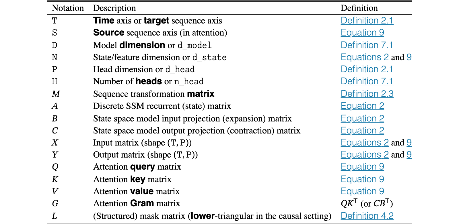
In this section we flesh out various algorithms for computing the scalar SSM scan, through the lens of structured matrix decompositions. The scalar SSM scan is defined as computing the recurrent part of the discrete SSM (7), in the case when $N=1$ (i.e. $A$ is a scalar). This is commonly used to compute SSMs recurrently; in particular, the case of structured SSMs where $A$ is diagonally structured reduces down to this operation, such as in the S5 (Smith et al., 2023) and S6 (Gu & Dao, 2023) models.

The goal of this section is to support a central theme of this paper that efficient algorithms for sequence models can be viewed as structured matrix multiplication algorithms. The various matrix decomposition ideas we show here are related to ideas used to derive fast SSM algorithms (Section 6), as well as directly used as a subroutine.

Let $a:\mathtt{(D,)}$ and $b:\mathtt{(D,)}$ be sequences of scalars. The scalar SSM scan is defined as

h_{t}=a_{t}h_{t-1}+b_{t}.

Here $h_{-1}$ can be an arbitrary value representing the previous hidden state to the SSM recurrence; unless otherwise specified, we assume $h_{-1}=0$ .

We also call equation (21) the cumprodsum (cumulative product sum). Note that the cumprodsum reduces to the cumprod (cumulative product) when $b=0$ is the additive identity and it reduces to the cumsum (cumulative sum) when $a=1$ is the multiplicative identity.

Finally, note that in vectorized form we can write

\begin{aligned}\displaystyle h & \displaystyle=Mb\end{aligned}

\begin{aligned}\displaystyle M & \displaystyle=\begin{bmatrix}1&\\ a_{1}&1&\\ a_{2}a_{1}&a_{2}&1\\ \vdots&\vdots&\ddots&\ddots\\ a_{T-1}\dots a_{1}&a_{T-1}\dots a_{2}&\dots&a_{T-1}&1\\ \end{bmatrix}\end{aligned}

In other words, this is simply the matrix-vector product by a 1-SS matrix $M$ .

Therefore we have three ways of viewing this fundamental primitive operation that are all equivalent:

•
A (scalar) SSM scan.
•
A cumprodsum.
•
A 1-SS matrix-vector multiplication .

We first describe the two classical ways of computing the SSM scan (21), previously used by prior work.

The recurrent mode simply computes (21) one timestep $t$ at a time. From the perspective of 1-SS multiplication, this was also described in Section 3.4.1.

Second, an important observation is that this recurrence can be turned into an associative scan (Martin & Cundy, 2018; Smith et al., 2023). This fact is not completely obvious. For example, S5 defined the correct associative scan operator and then showed associativity of the operator through rote calculation.

A slightly cleaner way to see that this is computable with an associative scan is to turn the multi-term recurrence into a single-term recurrence on a hidden state of size $2$ instead of $1$ :

\begin{aligned}\displaystyle h_{t} & \displaystyle=a_{t}h_{t-1}+b_{t}\end{aligned}

\begin{aligned}\displaystyle\begin{bmatrix}h_{t}\\ 1\end{bmatrix} & \displaystyle=\begin{bmatrix}a_{t}&b_{t}\\ 0&1\end{bmatrix}\begin{bmatrix}h_{t-1}\\ 1\end{bmatrix}.\end{aligned}

Then computing all the $h_{t}$ is the same as taking the cumulative products of these $2\times 2$ matrices. Since matrix multiplication is associative, this can be computed with an associative scan. The associative binary operator is simply matrix multiplication on these particular matrices:

\displaystyle\begin{bmatrix}a_{t}&b_{t}\\ 0&1\end{bmatrix}\begin{bmatrix}a_{s}&b_{s}\\ 0&1\end{bmatrix}=\begin{bmatrix}a_{t}a_{s}&a_{t}b_{s}+b_{t}\\ 0&1\end{bmatrix}.

Equating the top row yields the same associative scan operator as defined by S5:

(a_{t},b_{t})\otimes(a_{s},b_{s})=(a_{t}a_{s},a_{t}b_{s}+b_{t}).

The reason why associative scans are important is that they can be parallelized using a divide-and-conquer algorithm (Blelloch, 1990). We omit the details of this algorithm, and instead show that the entire associative SSM scan algorithm can be derived from scratch through matrix decompositions (Section B.3.5).

We discuss several algorithms for computing the SSM scan, all through the lens of finding structured matrix decompositions of the 1-SS matrix $M$ . These algorithms or computation modes include

•
A dilated mode where information is propagated $1,2,4,8,\dots$ steps at a time.
•
A state-passing mode where information is propagated forward in chunks.
•
A fully recurrent mode that increments one step at a time, which is a special case of the state-passing mode.
•
A block decomposition parallel mode where $M$ is divided into hierarchical blocks.
•
A scan mode where $M$ is divide into equal size blocks and reduced recursively.

This mode factors the 1-SS matrix in a particular way involving increasing “strides”. This is best illustrated through a concrete example:

\begin{aligned}\displaystyle M & \displaystyle=\begin{bmatrix}a_{0:0}&\\ a_{1:0}&a_{1:1}&\\ a_{2:0}&a_{2:1}&a_{2:2}\\ a_{3:0}&a_{3:1}&a_{3:2}&a_{3:3}\\ a_{4:0}&a_{4:1}&a_{4:2}&a_{4:3}&a_{4:4}\\ a_{5:0}&a_{5:1}&a_{5:2}&a_{5:3}&a_{5:4}&a_{5:5}\\ a_{6:0}&a_{6:1}&a_{6:2}&a_{6:3}&a_{6:4}&a_{6:5}&a_{6:6}\\ a_{7:0}&a_{7:1}&a_{7:2}&a_{7:3}&a_{7:4}&a_{7:5}&a_{7:6}&a_{7:7}\\ \end{bmatrix}\end{aligned}

\begin{aligned} & \displaystyle=\begin{bmatrix}a_{0:0}&\\ &a_{1:1}&\\ &&a_{2:2}\\ &&&a_{3:3}\\ a_{4:0}&&&&a_{4:4}\\ &a_{5:1}&&&&a_{5:5}\\ &&a_{6:2}&&&&a_{6:6}\\ &&&a_{7:3}&&&&a_{7:7}\\ \end{bmatrix}\begin{bmatrix}a_{0:0}&\\ &a_{1:1}&\\ a_{2:0}&&a_{2:2}\\ &a_{3:1}&&a_{3:3}\\ &&a_{4:2}&&a_{4:4}\\ &&&a_{5:3}&&a_{5:5}\\ &&&&a_{6:4}&&a_{6:6}\\ &&&&&a_{7:5}&&a_{7:7}\\ \end{bmatrix}\begin{bmatrix}a_{0:0}&\\ a_{1:0}&a_{1:1}&\\ &a_{2:1}&a_{2:2}\\ &&a_{3:2}&a_{3:3}\\ &&&a_{4:3}&a_{4:4}\\ &&&&a_{5:4}&a_{5:5}\\ &&&&&a_{6:5}&a_{6:6}\\ &&&&&&a_{7:6}&a_{7:7}\\ \end{bmatrix}\end{aligned}

Note that this closely resembles the computation of dilated convolutions.

We also note that this factorization shows that 1-SS matrices are a special case of butterfly matrices, another broad and fundamental type of structured matrix (Dao et al., 2019; Dao et al., 2020).

Remark 8.

This algoritihm is sometimes described as a “work-inefficient but more parallelizable” prefix sum algorithm (Hillis & Steele, 1986), becauses it uses $O(T\log(T))$ operations but has half the depth/span as the work-efficient associative scan algorithm.

This mode can be viewed as a generalization of the standard recurrent mode where instead of passing forward the recurrent state $h$ one step at a time, we compute the answer on chunks of arbitrary length $k$ and pass the state through the chunk. This can also be derived from a simple block decomposition of the 1-SS matrix.

Remark 9.

While we call this “state-passing” to refer to how states are passed from one local segment to another, this is related to the “chunkwise” algorithms proposed by related models (Sun et al., 2023; Yang et al., 2024).

Consider computing $h=Mb$ in “chunks”: for some index $k\in[T]$ , we want to compute $h_{0:k}$ or the output up to index $k$ , and have a way to reduce the problem to a smaller problem on indices $[k:T]$ .

We write $M$ as

\displaystyle M=\begin{bmatrix}a_{0:0}&\\ a_{1:0}&a_{1:1}\\ \vdots&&\ddots\\ a_{k-1:0}&\dots&\dots&a_{k-1:k-1}\\ a_{k:0}&\dots&\dots&a_{k:k-1}&a_{k:k}\\ \vdots&&&\vdots&\vdots&\ddots\\ a_{T-1:0}&\dots&\dots&a_{T-1:k-1}&a_{T-1:k}&\dots&a_{T-1:T-1}\\ \end{bmatrix}

Let the upper-left triangle be $M_{L}$ , lower-right be $M_{R}$ (left and right subproblems), and lower-left be $M_{C}$ . Divide up $b$ into $b_{L}=b_{0:k}$ and $b_{R}=b_{k:T}$ in the same way. Note that

\displaystyle Mb=\begin{bmatrix}M_{L}b_{L}\\ M_{R}b_{R}+M_{C}b_{L}\end{bmatrix}

Also, $M_{C}$ has the rank-1 factorization (this is essentially the defining property of semiseparable matrices)

\displaystyle M_{C}=\begin{bmatrix}a_{k:k}\\ \vdots\\ a_{T-1:k}\end{bmatrix}a_{k}\begin{bmatrix}a_{k-1:0}&\cdots&a_{k-1:k-1}\end{bmatrix}

Thus

\displaystyle M_{C}b_{L}=\begin{bmatrix}a_{k:k}\\ \vdots\\ a_{T-1:k}\end{bmatrix}a_{k}\cdot(Mb)_{k-1}.

Here we think of $(Mb)_{k-1}=h_{k-1}$ as the “final state” of the left chunk, because the row vector in $M_{C}$ ’s factorization is the same as the final row of $M_{L}$ . Furthermore, note that the column vector in $M_{C}$ ’s factorization is the same as the final column of $M_{R}$ . $^{7}$ Thus

\displaystyle M_{R}b_{R}+M_{C}b_{L}=M_{R}\begin{bmatrix}a_{k}h_{k-1}+b_{k}\\ b_{k+1}\\ \vdots\\ b_{T-1}\end{bmatrix}

Finally, we use the observation that $M_{L}$ and $M_{R}$ are self-similar to the original matrix $M$ ; the answers for these two smaller 1-SS matrix multiplications can be performed arbitrarily using any algorithm. In total, the algorithm proceeds as follows:

1.
Compute the left half of the answer $h_{0:k}$ using any desired method (i.e. any of the methods for 1-SS multiplication from this section).
2.
Compute the final state $h_{k-1}$ .
3.
Increment the state by one step to modify $b_{k}$ .
4.
Compute the right half of the answer $h_{k:T}$ using any desired method.

In other words, we compute the left subproblem as a black box, pass its final state on to the right problem, and compute the right subproblem as a black box.

The utility of this method comes from more complicated settings, such as in the general $N$ -semiseparable case, and when the input $b$ has an additional “batch” dimension (or in other words this is a matrix-matrix instead of matrix-vector multiplication). In this case, we can use an alternate algorithm for the chunks (corresponding to MM by $M_{L}$ and $M_{R}$ ) that does not materialize the full hidden states $h$ . Instead, we skip the hidden states and directly compute the final state $h_{k-1}$ in an alternate way, then “pass” the state to the next chunk.

This method can be very work-efficient because steps 2-3 takes only constant time. Therefore assuming the two subproblems (steps 1 and 4) are linear time, the whole method takes linear time.

The downside is that this is also sequential.

Note that the fully recurrent mode, where the recurrence is evolved one step at a time (21), is simply an instantiation of the state-passing mode with chunk size $k=1$ .

This uses the same matrix decomposition as the state-passing mode, but computes subproblems in a different order that trades off computation for parallelization.

As usual, we write $M$ as

\displaystyle M=\begin{bmatrix}1&\\ a_{1}&1&\\ a_{2}a_{1}&a_{2}&1\\ \vdots&\vdots&\ddots&\ddots\\ a_{T-1}\dots a_{1}&a_{T-1}\dots a_{2}&\dots&a_{T-1}&1\\ \end{bmatrix}=\begin{bmatrix}1&\\ -a_{1}&1&\\ 0&-a_{2}&1\\ \vdots&\vdots&\ddots&\ddots\\ 0&0&\dots&-a_{T-1}&1\\ \end{bmatrix}^{-1}

The key observation is again that the bottom-left quadrant of $M$ is rank-1. Aside from inspection, another way to see this is by using the RHS, observing that the bottom-left quadrant of it is a trivial rank-1 matrix (it is all 0 except the top-right corner is $-a_{T/2}$ ), and using the Woodbury inversion formula to see that the bottom-left corner of the LHS must also be rank 1. This also provides a way to deduce the rank-1 factorization, which can be verified through inspection:

\begin{aligned}\displaystyle M_{\text{lower-left-quadrant}} & \displaystyle=\begin{bmatrix}(a_{T/2}\dots a_{1})&\dots&a_{T/2}\\ \vdots&\ddots&\vdots\\ (a_{T-1}\dots a_{T/2}a_{T/2-1}\dots a_{1})&\dots&(a_{T-1}\dots a_{T/2})\end{bmatrix}\end{aligned}

\begin{aligned} & \displaystyle=\begin{bmatrix}a_{T/2}\\ \vdots\\ a_{T-1}\dots a_{T/2}\end{bmatrix}\begin{bmatrix}(a_{T/2-1}\dots a_{1})&\dots&a_{T/2-1}&1\end{bmatrix}.\end{aligned}

A second observation is that this matrix is self-similar: any principle submatrix has the same form. In particular, the top-left and bottom-right quadrants are both 1-SS matrices.

This provides an easy way to perform the matrix multiplication by $M$ : recurse on the two halves (i.e. top-left and bottom-right) in parallel, and then account for the bottom-left submatrix. This “combination” step in the divide-and-conquer algorithm is easy since the submatrix is rank 1. This leads to a parallel algorithm.

Like the state-passing algorithm, this method uses the same block decompositions of the rank-structured semiseparable matrices. The difference is that we recurse on both subproblems in parallel, while the state-passing algorithm handles the left and then right subproblems. This lowers the depth/span of the algorithm from linear to $\log(T)$ . The tradeoff is that the combination step (accounting for the rank-1 bottom-left submatrix) requires linear instead of constant work, so the total work is $O(T\log(T))$ instead of linear.

Note also that in the recursion, we can stop at any time and compute the subproblems in any other way. This is a main idea behind the SSD algorithm (Section 6), where we switch to the dual quadratic attention formulation on small subproblems.

The state passing (chunkwise) algorithm has linear work, but also involves sequential operations.

The block matrix reduction and dilated modes are parallelizable: they have $\log(T)$ depth/span. However, they do extra work ( $O(T\log(T)$ ).

As noted in Section B.2.2, there is an algorithm that achieves both $O(\log T)$ depth and $O(T)$ work by leveraging the associative scan (also called prefix scan) algorithm (Baker et al., 1996). This algorithm is most easily seen from the SSM scan or cumprodsum view, and even then is not obvious: it requires separately deriving an associative operator (22), and then leveraging the parallel/associative/prefix scan algorithm as a black box (Blelloch, 1990).

Here we show that it is actually possible to derive this parallel scan from leveraging a different matrix decomposition:

Nowweproceedinthreestages.

First we compute the answers for each of the diagonal blocks in the multiplication $Mb$ . This produces two numbers, but the first element is unchanged. For example, the second block is going to compute $b_{2}$ and $a_{3}b_{2}+b_{3}$

Now consider each of the $2\times 2$ blocks factored as a rank-1 matrix in the strictly lower triangular part of the matrix. Note that each of the right side row vectors is the same as the bottom row vector in the diagonal block in its column: in particular the $[a_{1:0}\;a_{1:1}]$ , $[a_{3:2}\;a_{3:3}]$ , and $[a_{5:4}\;a_{5:5}]$ rows.

Therefore we already have the answers to these from Stage 1, which is the second element of all $T/2$ subproblems in Stage 1. If we call this array of elements $b^{\prime}$ (of half the size of $b$ ), then we need to multiply $b^{\prime}$ by the 1-SS matrix generated by $a_{3:-1},a_{3:1},a_{5:3},a_{7:5}$ .

Finally, each of the answers to Stage 2 can be broadcast into two final answers by multiplying by the left-side column vectors: in particular the $[a_{2:2}\;a_{3:2}]^{\top}$ , $[a_{4:4}\;a_{5:4}]^{\top}$ , and $[a_{6:6}\;a_{7:6}]^{\top}$ vectors.

Note that this can be slightly modified with some off-by-one shifting of the indices. An equivalent way to view this algorithm is as the three-step matrix factorization

\begin{aligned}\displaystyle M & \displaystyle=\begin{bmatrix}a_{0:0}&\\ a_{1:0}&a_{1:1}&\\ a_{2:0}&a_{2:1}&a_{2:2}\\ a_{3:0}&a_{3:1}&a_{3:2}&a_{3:3}\\ a_{4:0}&a_{4:1}&a_{4:2}&a_{4:3}&a_{4:4}\\ a_{5:0}&a_{5:1}&a_{5:2}&a_{5:3}&a_{5:4}&a_{5:5}\\ a_{6:0}&a_{6:1}&a_{6:2}&a_{6:3}&a_{6:4}&a_{6:5}&a_{6:6}\\ a_{7:0}&a_{7:1}&a_{7:2}&a_{7:3}&a_{7:4}&a_{7:5}&a_{7:6}&a_{7:7}\\ \end{bmatrix}\end{aligned}

\begin{aligned} & \displaystyle=\begin{bmatrix}a_{0:0}&\\ &a_{1:1}&\\ &a_{2:1}&a_{2:2}\\ &&&a_{3:3}\\ &&&a_{4:3}&a_{4:4}\\ &&&&&a_{5:5}\\ &&&&&a_{6:5}&a_{6:6}\\ &&&&&&&a_{7:7}\\ \end{bmatrix}\begin{bmatrix}a_{0:0}&\\ &a_{1:1}&\\ &&a_{2:2}\\ &a_{3:1}&&a_{3:3}\\ &&&&a_{4:4}\\ &a_{5:1}&&a_{5:3}&&a_{5:5}\\ &&&&&&a_{6:6}\\ &a_{7:1}&&a_{7:3}&&a_{7:5}&&a_{7:7}\\ \end{bmatrix}\begin{bmatrix}a_{0:0}&\\ a_{1:0}&a_{1:1}&\\ &&a_{2:2}\\ &&a_{3:2}&a_{3:3}\\ &&&&a_{4:4}\\ &&&&a_{5:4}&a_{5:5}\\ &&&&&&a_{6:6}\\ &&&&&&a_{7:6}&a_{7:7}\\ \end{bmatrix}\end{aligned}

Note that Stage 1 and Stage 3 require $O(T)$ work, while Stage 2 reduces to a self-similar problem of half the size. It is easy to check that this requires $O(T)$ total work and $O(\log T)$ depth/span.

Remark 10.

In fact, it is possible to see that the computation graph of this algorithm is identical to that of the associative scan algorithm described in Section B.2.2. The key takeaway is that instead of the steps of (1) recognizing that $M$ defines a recurrence (2) observing that the recurrence can be defined with an associative binary operator; there is a completely different perspective of simply finding a structured matrix decomposition algorithm for $M$ .

We present here some additional properties of semiseparable matrices to illustrate their flexibility and utility. This section is not necessary to understand our core results.

Proposition C.1 (Semiseparable Closure Properties).

Semiseparable matrices are closed under several primitive operations.

•
Addition: The sum of an $N$ -SS and $P$ -SS matrix is at most ( $N+P$ )-SS.
•
Multiplication: The product of an $N$ -SS and $P$ -SS matrix is ( $N+P$ )-SS.
•
Inverse: The inverse of an $N$ -SS matrix is at most $(N+1)$ -SS.

The addition and multiplication properties are easily seen. The inverse property has many proofs; one approach follows immediately from the Woodbury inversion identity, which has also featured prominently in the structured SSM literature (Gu et al., 2022).

In turn, these imply closure properties of state space models.

For example, the addition property says that summing two parallel SSM models is still an SSM. The multiplication property says that sequentially composing or chaining two SSMs can still be viewed as an SSM, whose total state size is additive–a somewhat nontrivial fact.

Finally, the inverse property can let us relate SSMs to other types of models. For example, one can notice that banded matrices are semiseparable, so their inverses are semiseparable. (In fact, the semiseparable family of structure is often motivated by taking inverses of banded matrices (Vandebril et al., 2005)). Moreover, the fast recurrence properties of semiseparable matrices can be viewed as a consequence of their inverse being banded.

Remark 11.

The fact that 1-SS matrices are simple recurrences (7) are equivalent to the fact that the inverse of a 1-SS matrix is a 2-banded matrix:

\displaystyle M=\begin{bmatrix}1&\\ a_{1}&1&\\ a_{2}a_{1}&a_{2}&1\\ \vdots&\vdots&\ddots&\ddots\\ a_{T-1}\dots a_{1}&a_{T-1}\dots a_{2}&\dots&a_{T-1}&1\\ \end{bmatrix}=\begin{bmatrix}1&\\ -a_{1}&1&\\ 0&-a_{2}&1\\ \vdots&\vdots&\ddots&\ddots\\ 0&0&\dots&-a_{T-1}&1\\ \end{bmatrix}^{-1}

Thus $y=Mx\leftrightarrow M^{-1}y=x$ , or

\displaystyle\begin{bmatrix}1&\\ -a_{1}&1&\\ 0&-a_{2}&1\\ \vdots&\vdots&\ddots&\ddots\\ 0&0&\dots&-a_{T-1}&1\\ \end{bmatrix}y=x.

Or elementwise,

\begin{aligned} & \displaystyle y_{t}-a_{t}y_{t-1}=x_{t}\end{aligned}

\begin{aligned} & \displaystyle y_{t}=a_{t}y_{t-1}+x_{t}.\end{aligned}

Conversely, we also use these closure results to prove that autoregressive structured attention (under certain assumptions) must be SSMs, allowing us to show that more general families of efficient sequence models including attention variants can be reduced to state space models (Section C.2).

We prove Theorem 5.2 from Section 5.2. In Section 4.3 we defined structured attention as a broad generalization of masked attention, where the property of efficiency (i.e. a linear-time form for the kernel attention) is abstracted into the efficiency of structured matrix multiplication. However, beyond computational efficiency, standard linear attention (Katharopoulos et al., 2020) also has two important properties. First, it is causal, which is required for settings such as autoregressive modeling. Moreover, it has efficient autoregressive generation. In other words, the cost of an autoregressive step – i.e. the incremental cost of computing the output $y_{T}$ upon seeing $x_{T}$ , given that $x_{0:T}$ has already been seen and preprocessed – requires only constant time.

Here we characterize which instances of SMA have efficient autoregression.

In the framework of SMA, causality is equivalent to the constraint that the mask $L$ is a lower-triangular matrix.

Characterizing the space of $L$ matrices that have efficient autoregression is more difficult. We will use a narrow technical definition of autoregressive processes, in the spirit of classical definitions from the time series literature (e.g. ARIMA processes (Box et al., 2015)).

Definition C.2.

We define an autoregressive transformation $x\in\mathbb{R}^{T}\mapsto y\in\mathbb{R}^{T}$ of order $k$ as one where each output $y_{t}$ depends only on the current input and last $k$ outputs:

y_{t}=\mu_{t}x_{t}+\ell_{t1}y_{t-1}+\dots+\ell_{tk}y_{t-k}.

Note that the case where $L$ is the cumsum matrix is a special case with $k=1$ and thus $y_{t}=x_{t}+y_{t_{1}}$ . With this definition, characterizing the space of efficient autoregressive linear transforms follows from the properties of semiseparable matrices. Theorem C.3 formalizes and proves Theorem 5.2.

Theorem C.3.

Let $L\in\mathbb{R}^{T\times T}$ be an efficient autoregressive transformation of order $k$ . Then $L$ is a state space model of order $k+1$ .

Proof.

Let $(x,y)$ be input and output sequences, so that $y=Lx$ . Rearranging the definition (23),

\displaystyle y_{t}-\ell_{t1}y_{t-1}-\dots-\ell_{tk}y_{t-k}=\mu_{t}x_{t}.

Vectorizing over $t$ , this can be expressed as a matrix transformation

\displaystyle\begin{bmatrix}1&\\ -\ell_{t1}&1\\ \vdots&\ddots&\ddots\\ -\ell_{tk}&\dots&-\ell_{t1}&1\\ \vdots&\ddots&\vdots&\ddots&\ddots\\ 0&\dots&-\ell_{T-1,k}&\dots&-\ell_{T-1,1}&1\\ \end{bmatrix}\begin{bmatrix}y_{0}\\ y_{1}\\ \vdots\\ y_{k}\\ \vdots\\ y_{T-1}\\ \end{bmatrix}=\begin{bmatrix}\mu_{0}\\ &\mu_{1}\\ &&\ddots\\ &&&\mu_{k}\\ &&&&\ddots\\ &&&&&\mu_{T-1}\\ \end{bmatrix}\begin{bmatrix}x_{0}\\ x_{1}\\ \vdots\\ x_{k}\\ \vdots\\ x_{T-1}\\ \end{bmatrix}.

The $\mu$ diagonal matrix can be moved to the left and folded into the matrix of $\ell$ coefficients, which remains a $k+1$ -band lower-triangular matrix. But we also have $L^{-1}y=x$ , so $L$ is the inverse of this matrix.

Next, note that $k+1$ -band matrices are $k+1$ -semiseparable by the rank characterization of semiseparability (Definition 3.1). By Proposition C.1, the inverse $L$ is therefore at most $k+2$ -semiseparable. A slightly stronger bound of $k+1$ can be obtained because of the additional structure of banded matrices. Finally, the characterization of $L$ as an order- $k+1$ state space model follows from Theorem 3.5. ∎

In other words, efficient autoregressive attention is semiseparable SMA.

We use a harder version of the task introduced in Based (Arora et al., 2024a) where tokens that are not query/key/values are replaced with random tokens. We also use more key-value pairs, longer sequences, and smaller model sizes than the usual variant of MQAR used by prior work, all of which make the task harder.

For each sequence length $T\in\{256,512,1024\}$ , we use $T/4$ key-value pairs. The total vocab size is 8192.

We use a form of curriculum training where training cycles through datasets using $(T/32,T/16,T/8,T/4)$ key-value pairs, where each dataset has $2^{18}\approx 250000$ examples, for a total of $8$ epochs through each dataset (total of $2^{28}\approx 270M$ examples). The total batch size is $2^{18}\approx 0.25M$ tokens (e.g. for $T=1024$ , the batch size is $256$ ).

All methods use $2$ layers with default settings; the attention baseline additionally receives positional embeddings. For each method, we sweep over model dimensions $\mathtt{D}=\{32,64,128,256\}$ and learning rates $\{10^{-3.5},10^{-2},10^{-2.5}\}$ . We use a linear decay schedule that drops on every epoch (e.g. the last epoch would have a learning rate $1/8$ of the maximum/starting learning rate).

All models were trained on the Pile. For the scaling law experiments, we use the GPT2 tokenizer.

Table 7 specifies the model sizes we use for scaling laws following GPT3 (Brown et al., 2020), First, we changed the batch size of the 1.3B model from 1M tokens to 0.5M tokens for uniformity. Second, we changed the number of training steps and total tokens to roughly match Chinchilla scaling laws (Hoffmann et al., 2022), which specify that training tokens should increase proportionally to model size.

Original Table 7 — Table 7: (**Scaling Law Model Sizes**.) Our model sizes and hyperparameters for scaling experiments. (Model dimension and number of heads applies only to Transformer models.)

Table 7
Params	$\mathtt{n\_layers}$	$\mathtt{d\_model}$	$\mathtt{n\_heads}$ / $\mathtt{d\_head}$	Training steps	Learning Rate	Batch Size	Tokens
125M	12	768	12 / 64	4800	6e-4	0.5M tokens	2.5B
350M	24	1024	16 / 64	13500	3e-4	0.5M tokens	7B
760M	24	1536	16 / 96	29000	2.5e-4	0.5M tokens	15B
1.3B	24	2048	32 / 64	50000	2e-4	0.5M tokens	26B

All models used the AdamW optimizer with

•
gradient clip value $1.0$
•
weight decay $0.1$
•
no dropout
•
linear learning rate warmup with cosine decay

By default, the peak learning rate is the GPT3 specification.

Compared to GPT3 recipe, we use an “improved recipe”, inspired by changes adopted by popular large language models such as PaLM (Chowdhery et al., 2023) and LLaMa (Touvron et al., 2023). These include:

•
linear learning rate warmup with cosine decay to $1e-5$ , with a peak value of $5\times$ the GPT3 value
•
no linear bias terms
•
RMSNorm instead of LayerNorm
•
AdamW hyperparameter $\beta=(.9,.95)$ (the GPT3 value) instead of the PyTorch default of $\beta=(.9,.999)$

To evaluate downstream performance of fully trained, we train Mamba-2 on 300B tokens on the Pile, using the GPT-NeoX (Black et al., 2022) tokenizer.

We use the same hyperparameters as the scaling experiments, except with batch size 1M for the 1.3B and 2.7B model. For the 2.7B model, we also follow GPT3 specification (32 layers, dimension 2560).

For all models, we use 5x the learning rate of the corresponding GPT3 model.

For downstream evaluation, we use the LM evaluation harness from EleutherAI (Gao et al., 2021), on the same tasks as Mamba (Gu & Dao, 2023) with one additional one:

•
LAMBADA (Paperno et al., 2016)
•
HellaSwag (Zellers et al., 2019)
•
PIQA (Bisk et al., 2020)
•
ARC-challenge (Clark et al., 2018)
•
ARC-easy: an easy subset of ARC-challenge
•
WinoGrande (Sakaguchi et al., 2021)
•
OpenBookQA (Mihaylov et al., 2018)

Original Table 8 — Table 8: (**Zero-shot Evaluations**.) Best results for each size in bold, second best unlined. We compare against open source LMs with various tokenizers, trained for up to 300B tokens. Pile refers to the validation split, comparing only against models trained on the same dataset and tokenizer (GPT-NeoX-20B). For each model size, Mamba-2 outperforms Mamba, and generally matches Pythia at twice the model size.

Table 8
Model	Token.	Pile	LAMBADA	LAMBADA	HellaSwag	PIQA	Arc-E	Arc-C	WinoGrande	OpenbookQA	Average
		ppl $\downarrow$	ppl $\downarrow$	acc $\uparrow$	acc $\uparrow$	acc $\uparrow$	acc $\uparrow$	acc $\uparrow$	acc $\uparrow$	acc $\uparrow$	acc $\uparrow$
Hybrid H3-130M	GPT2	—	89.48	25.8	31.7	64.2	44.4	24.2	50.6	27.0	38.2
Pythia-160M	NeoX	29.64	38.10	33.0	30.2	61.4	43.2	24.1	51.9	29.2	39.0
Mamba-130M	NeoX	10.56	16.07	44.3	35.2	64.5	48.0	24.2	51.9	28.8	42.4
Mamba-2-130M	NeoX	10.48	16.86	43.9	35.3	64.9	47.4	24.2	52.1	30.6	42.6
Hybrid H3-360M	GPT2	—	12.58	48.0	41.5	68.1	51.4	24.7	54.1	31.6	45.6
Pythia-410M	NeoX	9.95	10.84	51.4	40.6	66.9	52.1	24.6	53.8	30.0	45.6
Mamba-370M	NeoX	8.28	8.14	55.6	46.5	69.5	55.1	28.0	55.3	30.8	48.7
Mamba-2-370M	NeoX	8.21	8.02	55.8	46.9	70.5	54.9	26.9	55.7	32.4	49.0
Pythia-1B	NeoX	7.82	7.92	56.1	47.2	70.7	57.0	27.1	53.5	31.4	49.0
Mamba-790M	NeoX	7.33	6.02	62.7	55.1	72.1	61.2	29.5	56.1	34.2	53.0
Mamba-2-780M	NeoX	7.26	5.86	61.7	54.9	72.0	61.0	28.5	60.2	36.2	53.5
GPT-Neo 1.3B	GPT2	—	7.50	57.2	48.9	71.1	56.2	25.9	54.9	33.6	49.7
Hybrid H3-1.3B	GPT2	—	11.25	49.6	52.6	71.3	59.2	28.1	56.9	34.4	50.3
OPT-1.3B	OPT	—	6.64	58.0	53.7	72.4	56.7	29.6	59.5	33.2	51.9
Pythia-1.4B	NeoX	7.51	6.08	61.7	52.1	71.0	60.5	28.5	57.2	30.8	51.7
RWKV4-1.5B	NeoX	7.70	7.04	56.4	52.5	72.4	60.5	29.4	54.6	34.0	51.4
Mamba-1.4B	NeoX	6.80	5.04	65.0	59.1	74.2	65.5	32.8	61.5	36.4	56.4
Mamba-2-1.3B	NeoX	6.66	5.02	65.7	59.9	73.2	64.3	33.3	60.9	37.8	56.4
GPT-Neo 2.7B	GPT2	—	5.63	62.2	55.8	72.1	61.1	30.2	57.6	33.2	53.2
Hybrid H3-2.7B	GPT2	—	7.92	55.7	59.7	73.3	65.6	32.3	61.4	33.6	54.5
OPT-2.7B	OPT	—	5.12	63.6	60.6	74.8	60.8	31.3	61.0	35.2	55.3
Pythia-2.8B	NeoX	6.73	5.04	64.7	59.3	74.0	64.1	32.9	59.7	35.2	55.7
RWKV4-3B	NeoX	7.00	5.24	63.9	59.6	73.7	67.8	33.1	59.6	37.0	56.4
Mamba-2.8B	NeoX	6.22	4.23	69.2	66.1	75.2	69.7	36.3	63.5	39.6	59.9
Mamba-2-2.7B	NeoX	6.09	4.10	69.7	66.6	76.4	69.6	36.4	64.0	38.8	60.2
GPT-J-6B	GPT2	–	4.10	68.3	66.3	75.4	67.0	36.6	64.1	38.2	59.4
OPT-6.7B	OPT	–	4.25	67.7	67.2	76.3	65.6	34.9	65.5	37.4	59.2
Pythia-6.9B	NeoX	6.51	4.45	67.1	64.0	75.2	67.3	35.5	61.3	38.0	58.3
RWKV4-7.4B	NeoX	6.31	4.38	67.2	65.5	76.1	67.8	37.5	61.0	40.2	59.3

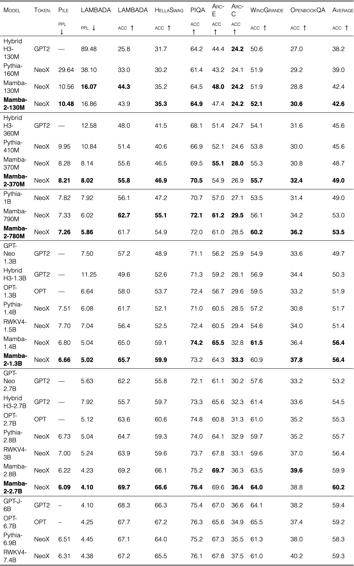
Our ablations in Section 9.4.3 considered the Based (Arora et al., 2024a) and ReBased (Aksenov et al., 2024) models.

Based approximates the $\exp$ kernel with a quadratic Taylor expansion $\exp(x)\approx 1+x+x^{2}/2$ , which can be accomplished by the feature map

\psi_{\text{Taylor}}(x)=\mathsf{concatenate}(1,x,1/\sqrt{2}x\otimes x).

ReBased proposes to use the simpler feature map $\psi_{\text{Quadratic}}(x)=x\otimes x$ corresponding to the kernel transformation $x^{2}$ , but also applies a layer normalization beforehand. We view the layer normalization as an alternative non-linear activation to our default Swish activation, and ablate combinations of these.

Note that because these expand the feature dimension, we must project to smaller $B,C$ dimensions; in Figure 12, use state size $N=64$ for 130M models and $N=256$ for 380M models. For the (Re)Based methods, we project to 8 and 16 dimensions respectively before applying their feature maps; this results in a total state size of $8^{2}=64$ for ReBased and $1+8+8^{2}=73$ for Based in the 130M model case. Because the $B$ and $C$ projections are smaller, these methods use fewer parameters, and we adjust the layer count appropriately.

Transformers are SSMs: Generalized Models and Efficient Algorithms Through Structured State Space Duality

Abstract

References

Meow summary

The problem

The trick: two routes to the same answer

Why it helps

Where it stops

Make notes of your own

Abstract

1 Introduction

State Space Duality.

Efficient Algorithms.

Architecture Design.

Systems Optimizations.

2 Background and Overview

2.1 Structured State Space Models

Continuous-time Models.

Recurrent Models.

Convolutional Models.

Selective State Space Models.

Structured SSMs as Sequence Transformations.

2.2 Attention

2.3 Structured Matrices

2.4 Overview: Structured State Space Duality

Recurrent (Linear) Form.

Dual (Quadratic) Form.

Matrix Form and SSD Algorithm.

2.5 Notation

Matrices and Vectors.

Indexing.

Dimensions.

Tensor Contractions.

3 State Space Models are Structured Matrices

3.1 The Matrix Transformation Form of State Space Models

3.2 Semiseparable Matrices

3.2.1 The Sequentially Semiseparable (SSS) Representation

3.2.2 1-Semiseparable Matrices: the Scalar SSM Recurrence

3.3 State Space Models are Semiseparable Matrices

3.4 Computing State Space Models through Structured Matrix Algorithms

3.4.1 The Linear (Recurrent) Mode

3.4.2 The Quadratic (Naive) Mode

3.4.3 Summary

4 Structured Masked Attention: Generalizing Linear Attentionwith Structured Matrices

4.1 The Attention Framework

4.1.1 Attention

4.1.2 Self-Attention

4.1.3 Kernel Attention

4.1.4 Masked (Kernel) Attention

4.2 Linear Attention

4.2.1 A Tensor Contraction Proof of Linear Attention

4.3 Structured Masked Attention

4.3.1 Summary: The Dual Forms of Masked Attention

5 State Space Duality

5.1 Scalar-Identity Structured State Space Models

5.2 1-Semiseparable Structured Masked Attention

5.3 Structured State-Space Duality (SSD)

6 A Hardware-Efficient Algorithm for SSD Models

6.1 Diagonal Blocks

6.2 Low-Rank Blocks

Right Factors.

Center Factors.

Left Factors.

6.3 Computational Cost

Center Blocks.

Low-Rank Blocks: Right Factors.

Low-Rank Blocks: Center Factors.

Low-Rank Blocks: Left Factors.

Total Cost.

Comparison to Pure SSM and Attention Models.

7 The Mamba-2 Architecture

7.1 Block Design

Parallel Parameter Projections.

Extra Normalization.

7.2 Multihead Patterns for Sequence Transformations

Multihead SSM (MHS) / Multihead Attention (MHA) Pattern.

Multi-contract SSM (MCS) / Multi-query Attention (MQA) Pattern.

Multi-input SSM (MIS) / Multi-value Attention (MVA) Pattern.

Grouped Head Patterns.

7.3 Other SSD Extensions from Linear Attention

Kernel Attention Approximations to Softmax Attention.

Exponential Kernel Feature Maps.

Incorporating a Normalization (Denominator) Term.

8 Systems Optimization for SSMs

8.1 Tensor Parallel

8.2 Sequence Parallelism

8.3 Variable Length

9 Empirical Validation

9.1 Synthetics: Associative Recall