The Surprising Effectiveness of Test-Time Training for Few-Shot Learning
arXiv:2411.07279v2 · This workspace stays on this version. Check arXiv for newer versions
Some source details need review 1 to check
Original formulas, table values and figures are preserved. Comparison can miss differences; use the original PDF to check details.
Reading view checked: 221 math expressions, 0 rendering failures; 28 of 28 images available.
Compared 159 of 159 source passages against 22 of 22 PDF pages.
- An unsupported comparison claim was rejected; source verification is incomplete.
28 of 28 figure, table and graphic images captured. Open original PDF
Abstract
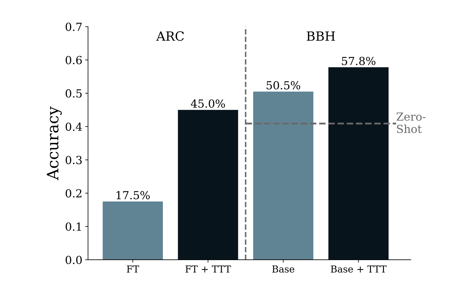
Language models (LMs) have shown impressive performance on tasks within their training distribution, but often struggle with structurally novel tasks even when given a small number of in-context task examples. We investigate the effectiveness of test-time training (TTT)—temporarily updating model parameters during inference using a loss derived from in-context examples—as a mechanism for improving LMs’ reasoning and few-shot learning capabilities. On the Abstraction and Reasoning Corpus (ARC), performing TTT with in-context examples yields up to higher accuracy compared to fine-tuned baselines—reaching on the public validation set with an 8B-parameter LM and when ensembled with program-synthesis methods, matching average human performance. On BIG-Bench Hard (BBH), TTT on in-context examples surpasses standard few-shot prompting in the -shot setting by percentage points ( to ). Our findings highlight the limitations of in-context learning for novel tasks and demonstrate the potential of test-time training to enhance language model adaptability.
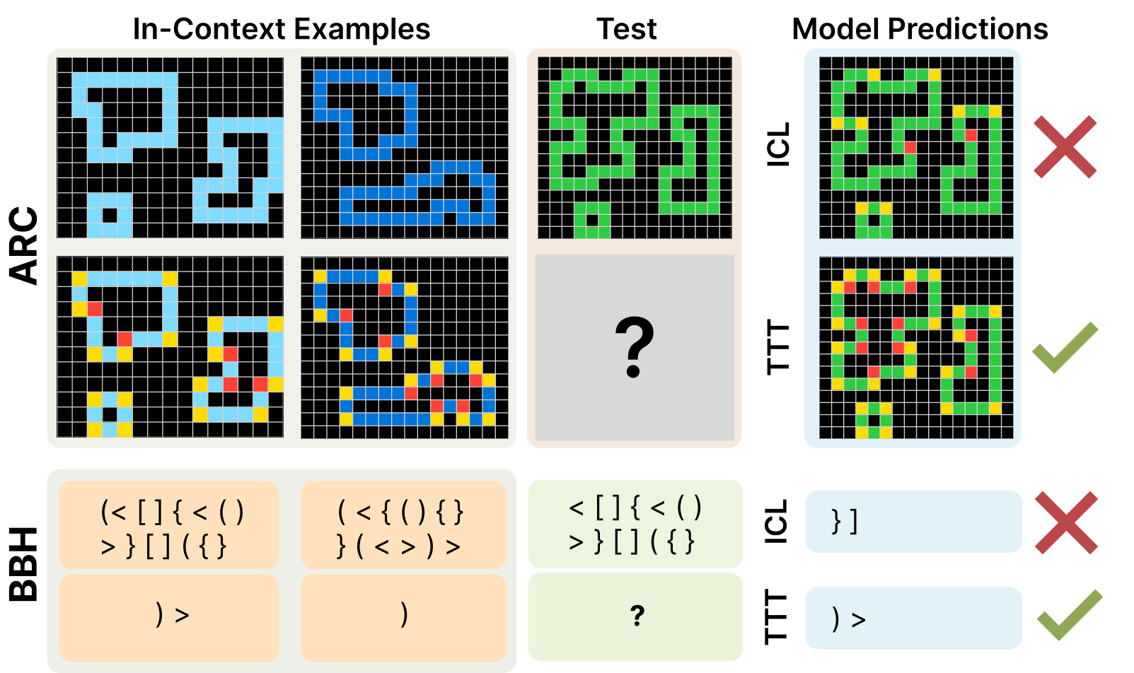
Large-scale neural language models (LMs) have demonstrated remarkable success on few-shot learning of tasks related to those seen during pre-training, as well as elementary variations or compositions of those tasks (Brown et al., 2020; Todd et al., 2024). When given natural language specifications or a small number of examples, LMs can often infer the desired task and generate appropriate outputs. However, an open question is whether these models can truly acquire new skills for which they have not been trained—particularly, tasks involving non-trivial reasoning, planning, and abstraction in domains that differ significantly from their pre-training distributions. This question is fundamental to understanding how, and whether, LMs can exhibit the sort of flexible, novel-skill acquisition that has been proposed as a measure of intelligence (Chollet, 2019).
Solving complex and novel tasks remains extremely challenging for LMs, and simple sampling approaches often yield poor performance on such problems (Wu et al., 2024; McCoy et al., 2024). However, recent progress has shown that LMs can be substantially improved by adding extra test-time computation. Several methods fall into this category, such as chain-of-thought prompting (Wei et al., 2022), sampling with majority voting (Wang et al., 2023, self-consistency;), code execution (Brown et al., 2024; Snell et al., 2025; Damani et al., 2025), and search (Yao et al., 2023).
The idea of updating model parameters using instance-specific data at test time has roots in the literature on local learning (Bottou & Vapnik, 1992) and transductive learning (Joachims, 1999). In these methods, a learner refines its parameters or hypotheses after observing test inputs, adapting to individual examples or small clusters of examples. Such approaches inherently blur the line between training and inference, and can lead to robust adaptation in low-data scenarios or under distribution shift.
Modern versions of these transductive ideas for deep neural networks have been widely referred to as test-time training. In TTT, a model is updated at inference time using only the current test instance or a small batch of test instances, typically through explicit gradient steps. While test-time adaptation has been explored for vision models (Sun et al., 2020) and sequence architectures (Gandelsman et al., 2022; Sun et al., 2024; Behrouz et al., 2025), its interaction with other techniques for few-shot learning—especially in-context learning—remains less understood.
In this paper, we investigate how to leverage TTT on top of standard in-context learning (ICL) to boost performance on challenging tasks that require reasoning or rule-based generalization. In-context learning is a powerful means of adaptation without parameter updates, guided by short, task-specific prompts. We show that combining ICL with explicit gradient-based updates on test data can significantly improve performance on particularly difficult tasks. Specifically, our main contributions are:
- 1.
A systematic analysis of the key components for effective test-time training, including strategies for selecting training data at inference, training objectives, and how TTT interacts with an LM’s pre-trained parameters and in-context learning.
- 2.
An application of TTT to two challenging benchmark suites—The Abstraction and Reasoning Corpus (ARC; Chollet, 2019) and BIG-Bench Hard (BBH; Srivastava et al., 2023; Suzgun et al., 2023).
On ARC, our TTT approach outperforms existing open-source neural methods, attaining % accuracy with an 8B model and % when ensembled with a program-synthesis approach (comparable to human performance). On BBH, TTT yields a % absolute improvement over few-shot prompting, achieving % accuracy. Gains are particularly large on tasks involving structural rules or distribution shifts (e.g., Dyck languages, Ruin names), where TTT yields 20–50 percentage points of improvement over standard in-context prompting.
Overall, our findings highlight that TTT drastically improves LM’s few-shot learning ability on out-of-distribution tasks.
At a certain scale, many LMs exhibit the ability to adapt to new tasks without updating their parameters by simply conditioning on input examples or instructions provided. Given a sequence of input-output pairs and a new input , an LM can generate the corresponding output by sampling from:
While the possibility of in-context learning (ICL) as implicit machine learning simulation is discussed in previous work (Akyürek et al., 2023), empirical evidence shows that in-context learning with language models does not always resemble standard machine learning algorithms (Zhao et al., 2024; Min et al., 2022b). Furthermore, ICL often struggles with novel tasks “out-of-the-box.” For example, large language models exhibit poor performance on datasets like ARC (Opiełka et al., 2024; Bober-Irizar & Banerjee, 2024).
Test-time training (TTT) enables parametric models to adapt during inference through dynamic parameter updates in response to each test input. This approach remains relatively unexplored in the era of large language models. The general TTT process is as follows: starting with initial model parameters , for each test input (or batch of inputs) , we generate a temporary training dataset . We then optimize these parameters to minimize a loss function
resulting in temporarily updated parameters , which are subsequently used for prediction.
In previous work (Sun et al., 2020, e.g.,), is typically constructed by applying an unsupervised objective (e.g., masked autoencoding) to the input alone. In this paper, we extend TTT to the few-shot learning setting, treating it as a form of transductive learning by leveraging few-shot demonstration examples to improve predictions. Although TTT can also be applied to chain of thought (Wei et al., 2022, CoT;), we focus on direct transduction, where demonstrations consist of input-output pairs without intermediate reasoning steps or explicit function descriptions.
The few-shot learning setting we consider provides richer context in the form of demonstration pairs . One simple method for TTT is Direct I/O training, where we directly treat each input-output pair as training instances. Our key insight is that the few-shot examples can also be used to construct a more robust and expansive of synthetic in-context learning tasks, allowing for effective model adaptation during test time. Additionally, when task-specific knowledge is available, this structure can be leveraged to further expand the dataset, as demonstrated in our experiments on ARC (Section 4). We also explore the general case where no task-specific information is used, as tested on BBH (Section 5).
Our experiments in this paper characterize each component of the TTT pipeline, investigating different design choices across the following stages: (1) constructing an input-specific training dataset at test-time; (2) fine-tuning the LM by optimizing a loss function over the dataset ; and (3) sampling from the updated model with an augmented inference strategy based on self-consistency to obtain a final prediction.
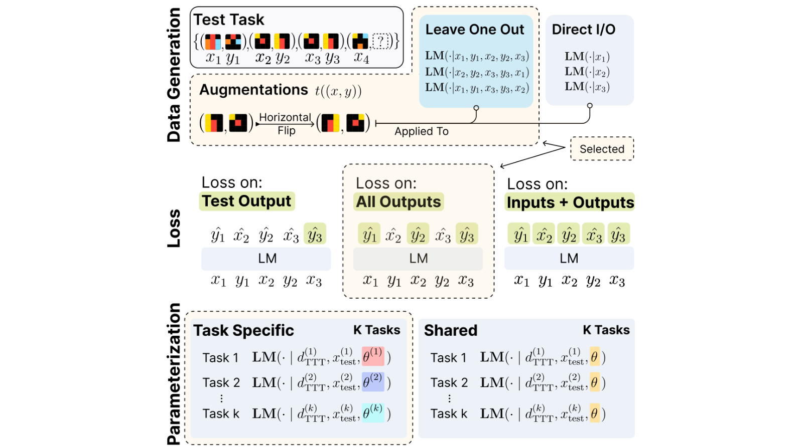
This section discusses the key design choices and challenges of applying TTT to LLMs, including how to best leverage their in-context learning capabilities, how to structure data for effective processing, what optimization objective to use, and how to efficiently update model parameters. We detail these considerations in the construction of the TTT dataset and the optimization setup (Figure 2).
Given a task with training input-output pairs , a test-time training dataset can be created by either following an in-context learning setup or a direct input-output (direct I/O) setup (top row in Figure 2):
We begin with leave-one-out in-context learning tasks. For each pair , we exclude it from the set of demonstrations and treat it as a “test” example within the newly formed synthetic task:
Here, serves as the “in-context demonstrations,” and is the “synthetic test example.” To increase the number of synthetic tasks, we additionally permute the order of the demonstrations in each .
Rather than constructing in-context tasks, we treat each pair independently as a single training instance:
In this setup, the model is fine-tuned on these training pairs without in-context demonstrations. While this approach is more computationally efficient, our results (Sections 4 and 5) show that it underperforms methods that utilize in-context demonstrations.
Data augmentation For certain tasks with structured inputs (e.g., ARC), we can apply invertible transformations (e.g., flips, rotations, color permutations) to further augment the TTT dataset. Let be a set of invertible transformations. For each , we have , so we can apply to each training and test instance in to yield a transformed task . Since these transformations preserve the core relationships in the data (e.g., the input-output pattern is the same, just rotated), they effectively expand the training signal. If rule-based transformations are used, the final TTT dataset is:
We optimize the standard LM loss on . For the in-context leave-one-out setup, we experiment with different ways to take the loss (middle row in Figure 2):
- •
Test output (no demonstration loss) The standard formulation where the loss is taken over :
- •
All outputs In addition to the loss on the test output, the loss is also taken over the outputs of the in-context demonstrations, which encourages the model to correctly predict the demonstration outputs after seeing the previous demonstrations:
- •
Loss on inputs and outputs The loss is taken over all tokens, encouraging the model to learn the structure of as well as :
This method, which requires learners to generate task inputs as well as outputs, is analogous to existing unsupervised TTT objectives (Sun et al., 2020).
We find in Sections 5.3 and 4.3 that the first method (taking the loss over both demonstration and test outputs) works best.
Once we have the test-time training dataset (constructed via either the in-context or direct I/O approach), we perform a small number of gradient steps on task-specific LoRA adapters (Hu et al., 2022). This approach allows computationally efficient adaptation while maintaining the model’s general capabilities. By default, we learn task-specific LoRA adapters for each ARC or BBH task at test-time. That is, we obtain different LoRA adapters, where is the number of test tasks. We also experiment with using a single shared LoRA adapter from the aggregated dataset of few-shot examples drawn from multiple tasks (bottom row in Figure 2)—a test-time version of meta-ICL (Min et al., 2022a). We find that the shared adapter degrades performance on ARC, whereas it improves performance on BBH. We discuss this in more detail in Section 5.3.
The Abstraction and Reasoning Corpus (ARC) aims to evaluate the abstract reasoning capabilities of language models through their ability to solve visual puzzles. Each puzzle (henceforth referred to as a task) consists of input-output pairs of 2D grids (up to in size) containing shapes or patterns in up to different colors, as displayed in Figure 3. The output of each pair is obtained by applying an intuitive and shared transformation or rule . Each task has 2-7 demonstration examples and 1-3 test examples.
For our ablation experiments, we use the 1B-parameter Llama-3.2 model (Llama Team, 2024). For our final results in Section 4.6, we use the 8B Llama 3 model. We use Low-Rank Adaptation (Hu et al., 2022, LoRA;) for parameter-efficient test-time training. More details are given in Section C.2.
While TTT offers task-specific adaptation, the initial capabilities of the base model significantly influence its final performance (Section 4.4). We developed several approaches for generating synthetic training data to enhance the base model’s abstract reasoning capabilities through fine-tuning, exploring both automated and semi-automated methods for task generation. This is complementary to TTT as the base model is fine-tuned on tasks distinct from those tested on, when TTT is applied. Details on our data generation strategies, as well as the effects of various data sources and model sizes on performance, are provided in Appendix B. The fine-tuned base model serves as the foundation for all subsequent experiments.
The success criterion requires producing an exact match for all test outputs (no partial credit). Following the standard ARC scoring criteria, we use the pass@2 metric and produce attempts for each test input. The original training and validation sets consist of tasks each. However, for efficient evaluation purposes, we randomly pick balanced ARC tasks from the ARC validation set, including easy, medium, hard, expert tasks according to the classification in (LeGris et al., 2024) (see Table 2 for this task list). Except for our final results, we use this subset of ARC tasks throughout our experiments. We limit to have a maximum of examples per task for efficiency reasons. Section C.2 provides additional details on the hyperparameters.
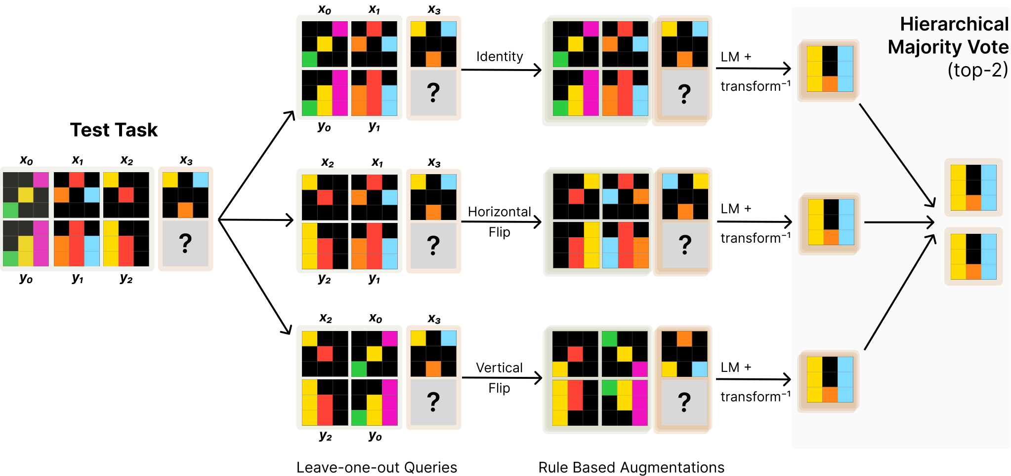
One of the most common techniques to scale inference-time compute is to use temperature sampling to obtain multiple responses and select the best according to a ranker, called self-consistency (Wang et al., 2023). However, this is not viable in ARC (where the output grid is directly predicted) as there is no way to directly enforce diversity across samples while ensuring coherence within samples. As an alternative self-consistency approach, we try an augmented inference strategy that combines greedy decoding with multiple versions of the input. Specifically, we generate multiple prediction candidates by using geometric transformations. We then employ a hierarchical voting strategy to determine the final prediction from the set of generated candidates. This approach involves two stages of voting to progressively narrow down the best candidates: (1) Intra-transformation voting: Group predictions by their corresponding transformation . Within each group, select the top-3 most frequent predictions. (2) Global voting: Take the selected transformation-specific candidates from the previous step and select the top-2 most frequent predictions across all transformations. The augmented inference pipeline is summarized in Figure 4 and full details of the pipeline are in Appendix E.
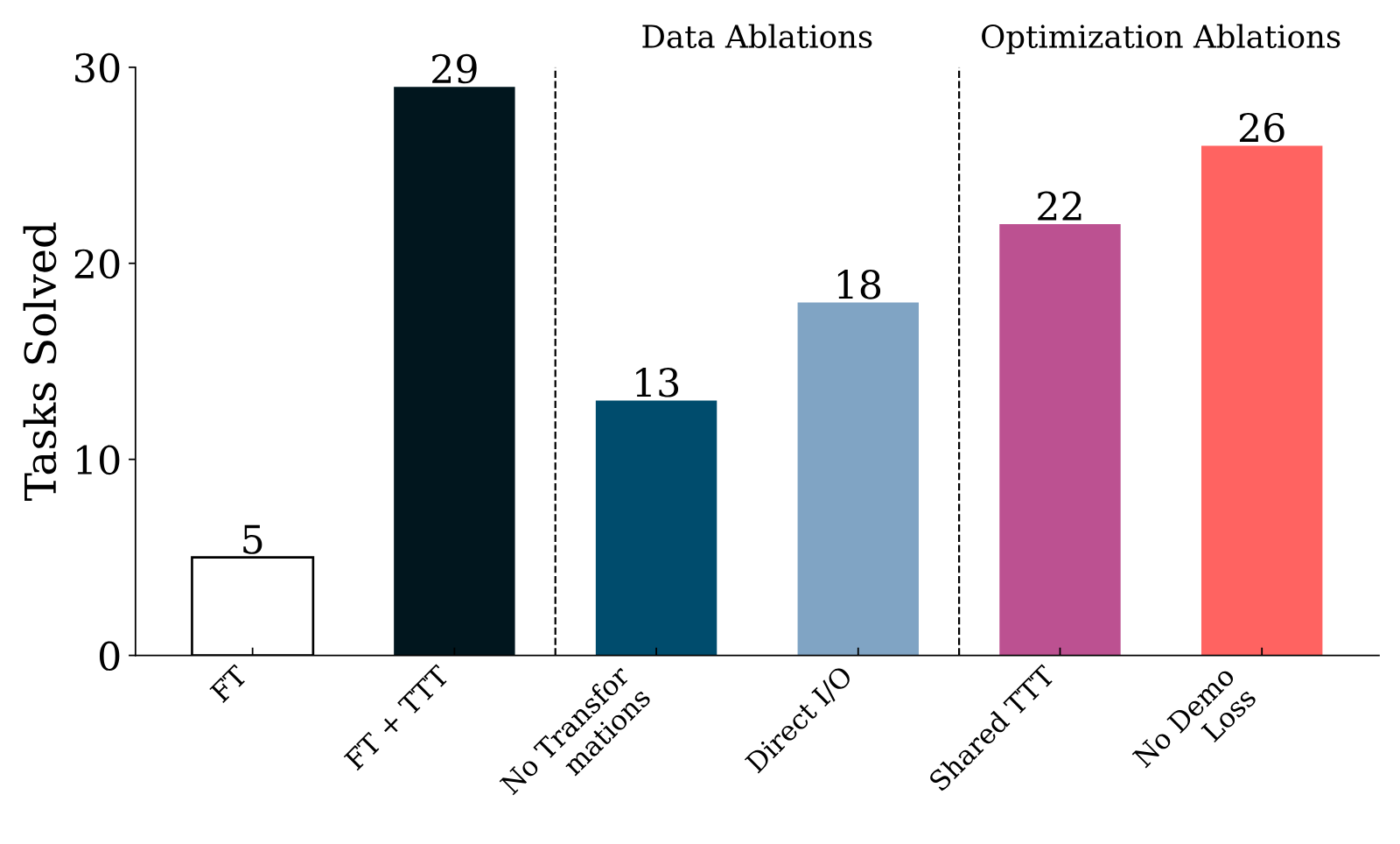
In this section, we compare the final implementation of our method with different design choices for TTT. FT serves as the baseline, using only the fine-tuned model with demonstrations in-context. No Transformations omits the augmentation step. Direct I/O Data replaces in-context tasks with the direct input-output task formulation (Section 3.1). Shared TTT uses a single LoRA adapter across all tasks instead of learning one per task. No Demonstration Loss removes the loss on demonstration outputs (Section 3.1).
Results are presented in Figure 5. Our TTT method is effective, improving fine-tuned model accuracy approximately 6 . In-context formatting is especially important; using the direct input-output data to construct causes an -task drop (). Removing transformations causes a task drop (). Regarding optimization, per-task LoRA adapters outperform a single shared adapter by tasks (). Including losses on the demonstration outputs yields a modest but consistent gain ().
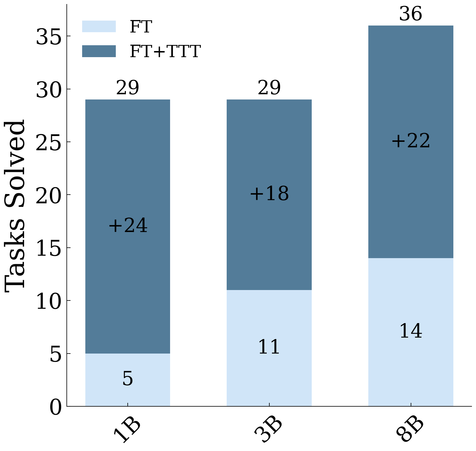
We perform full fine-tuning of 1B and 3B Llama 3.2 (instruction-tuned) and 8B Llama 3 (instruction-tuned) using synthetically generated data, as detailed in Appendix B, and then use our default TTT implementation. We show results using different model sizes in Figure 6. Increasing the model size consistently improves FT performance, with the 8B model achieving the highest accuracy of . At all model sizes, TTT leads to significant improvements in performance. We also observe that for smaller model sizes, TTT effectively closes the performance gap, with the 1B and 3B models achieving similar accuracy after TTT.
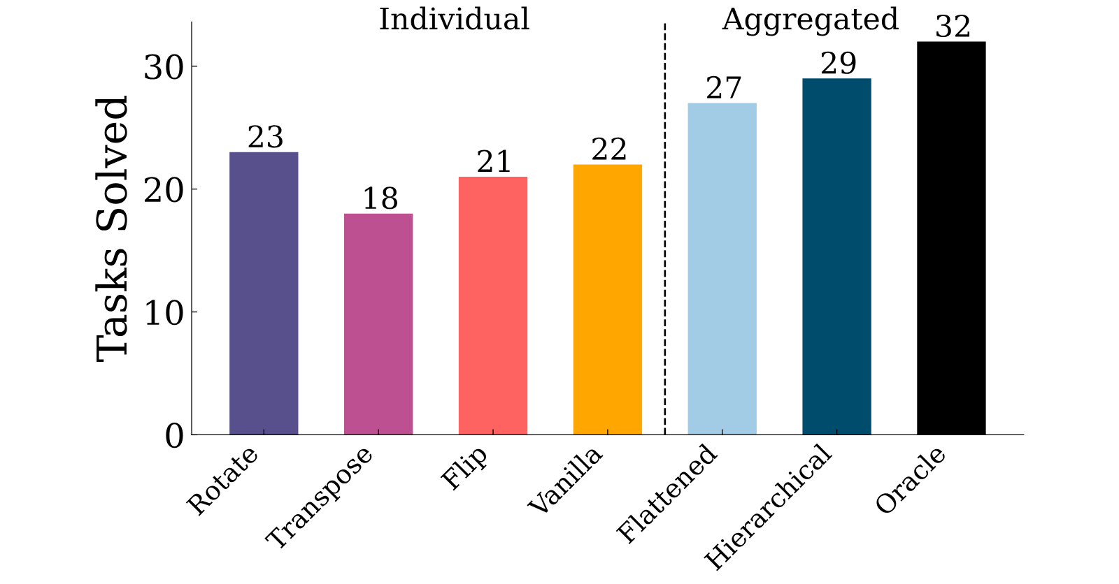
To analyze the impact of augmented inference and voting, we run several ablations: (1) Vanilla, which generates two predictions without transformations or advanced voting; (2) Transformed Inference, applying a single transformation (Rotate, Transpose, or Flip) to measure its isolated effect; (3) Hierarchical Voting, our full pipeline combining augmented inference and structured voting; (4) Flattened Voting, which selects the top-2 predictions from a single voting round over all generated outputs; and (5) Oracle, an upper bound that selects the correct answer if present.
As shown, individual transformations are modestly effective on their own (with Transpose performing worst), but their aggregation improves results markedly. Hierarchical voting further outperforms a flattened voting approach and closely approaches the oracle’s accuracy, suggesting that our two-stage aggregation effectively identifies the correct solution when it is present.
Following our experiments on tasks, we present comprehensive results on the full ARC public evaluation set, comparing our system against existing approaches. Our analysis focuses on three key aspects: the impact of our TTT methodology, the benefits of combining our approach with existing methods, and the differences between fully neural and program synthesis methods.
We apply TTT and augmented inference procedure to our base fine-tuned model (fine-tuned 8B model). TTT significantly improves accuracy from % to %.
| PS | Fine-tuned LM | TTT Method | Score |
| X | Ours | X | % |
| X | Ours | Ours | % |
| X | BARC | Ours | % |
| BARC | Ours | Ours | % |
| BARC | BARC | Ours | % |
| Avg. Human | % | ||
| Best Human | % | ||
| BARC (ensemble) | % | ||
| BARC (no synthesizer) | % | ||
| Claude 3.5 Sonnet | % | ||
| GPT-4o | % | ||
| OpenAI o1 preview | % | ||
| DeepSeek r1 | % | ||
| OpenAI o3 | % | ||
View original table
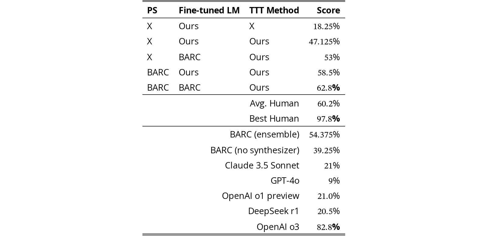
A concurrent work by Li et al. (2025) introduced BARC, achieving % accuracy by combining neural and program synthesis approaches. While their fully neural approach shares similarities with our system, our TTT and inference pipeline has several additional components (per-task LoRA, more augmentations, hierarchical voting) that boost performance. To validate our improvements, we applied our TTT pipeline to BARC’s fully neural model, achieving accuracy—a improvement over their original TTT method.
Building on these results, we explored combinations of our approach with BARC. Combining our TTT pipeline and neural model with BARC’s synthesizer raised accuracy to %. Combining our TTT pipeline with BARC’s neural model and synthesizer raised accuracy to %. This configuration matches average human performance of (LeGris et al., 2024) on the benchmark.
Li et al. (2025) found that program synthesis and fully neural predictors for ARC are highly complementary. Their end-to-end neural model can only solve of the tasks solved by the program synthesis model. However, we find that when equipped with our TTT pipeline, BARC’s fine-tuned fully neural model solves of the tasks that are solved by the program synthesis model. This suggests that our TTT pipeline significantly improves the neural model’s ability to learn systematic reasoning patterns similar to those captured by program synthesis models.
ARC-AGI challenge provides a hidden “semi-private dataset” and performs external tests for submissions. We submitted our ensemble solution to the official ARC-AGI semi-private evaluation and observed % accuracy. This decline may be attributed to more significant distribution shifts in the semi-private evaluation dataset. If the semi-private evaluation results become publicly available in future, we will provide a detailed analysis of these performance differences.
BIG-Bench Hard (Srivastava et al., 2023; Suzgun et al., 2023, BBH;) is a benchmark comprising challenging tasks across task types, designed to evaluate large language models on reasoning, compositionality, and generalization. Unlike ARC, BBH features a broader natural language structure and lacks a shared input format, making it unsuitable for invertible transformations. However, this broader scope offers a valuable testbed for evaluating TTT’s effectiveness in a more generalized setting. Despite the absence of invertible transformations—previously used in ARC to expand the TTT dataset and enhance inference—TTT still significantly improves performance on BBH.
We use Llama 3.1 (Llama Team, 2024, 8B;). For each task , we train a separate set of LoRA parameters at test-time, with a LoRA rank of over random shuffles of the demonstration pairs to produce leave-one-out in-context tasks. More hyperparameter details are given in Section F.1.
On BIG-Bench Hard, our base language model is able to achieve non-trivial scores out-of-the-box. Consequently, we do not perform any initial fine-tuning on synthetic tasks outside of BBH like we do for ARC. Furthermore, since models achieve nonzero performance in a zero-shot setting, we provide the zero-shot results and analyze how TTT and ICL improve upon them.
For the tasks in BBH, we consider the -shot setting, where we select random pairs from each task’s dataset to be demonstration pairs and evaluate on the remaining data. Each of the tasks is analogous to a single ARC task, consisting of labeled examples as demonstration pairs given at test-time. We report average results over five random seeds, where each seed specifies which examples form the demonstration subset. For more control over the evaluation process with test-time training, we write our own evaluation function, which is available in our codebase (for more details, see Section F.1). The number of evaluation examples for each task is then for all tasks except three: Causal Judgment, Penguins in a Table, and Snarks, which have , , and evaluation examples respectively. Note that the large number of evaluation samples for each task compared to ARC means we can do a task-specific analysis to analyze which types of tasks benefit the most from TTT (Section 5.4). Unlike with ARC, we do not have a collection of invertible transformations to run augmented inference. Instead, we use greedy decoding. Further hyperparameter details and evaluation details are given in Section F.2.
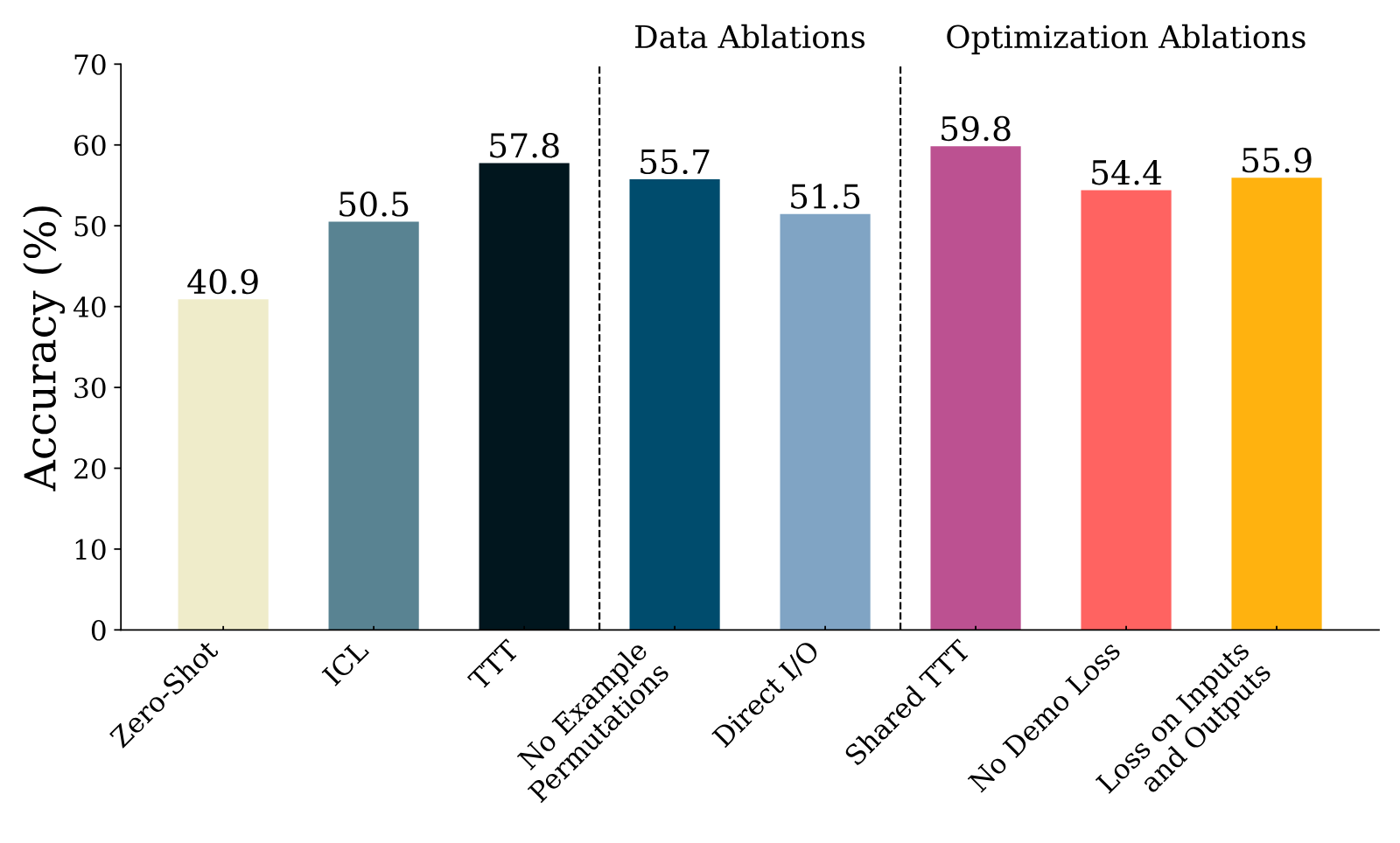
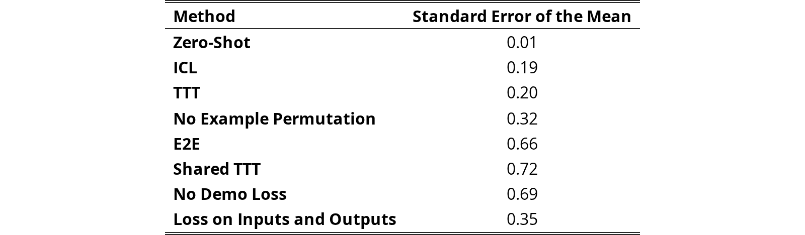
In this section, we evaluate our method and its ablations, primarily comparing the zero-shot baseline, ICL, and TTT. No Example Permutation updates the model on a single in-context prompt instead of multiple shuffled versions. Direct I/O treats each input-output pair as separate training instances. Shared TTT uses a single adapter across tasks instead of task-specific adapters. No Demonstration Loss removes the loss applied to demonstration outputs. Loss on Inputs and Outputs extends the loss calculation to both inputs and outputs. These ablations are as detailed in Section 3. As these results are averages over runs, the standard errors of the mean for each method are given in Section F.1, averaging .
The results in Figure 8 show that TTT achieves an overall accuracy of %, outperforming standard ICL (%) and Direct I/O learning (%). This demonstrates that TTT’s capabilities extend beyond ARC to more diverse and complex reasoning tasks, proving its effectiveness in a broader range of natural language problem-solving scenarios.
We observe that TTT without example permutations—performing multiple gradient steps on a single in-context prompt before inference—reduces accuracy to a still-impressive . Computing the loss only on the test output lowers accuracy to , while applying it to both inputs and outputs achieves
Unlike on ARC, using a shared adapter improves performance on BBH, indicating that tasks in BBH do not confound each other during training. On the ARC dataset, each puzzle has the same input format, so distinguishing among multiple tasks is difficult, and we may have conflicting gradients with a single adapter. In BBH, however, distinguishing tasks is trivial (the instructions differ in plain text), and many tasks are mutually helpful. For instance, updating on Logical Deduction Five Objects also aids Logical Deduction Three Objects, without hurting Word Sorting. Although this is no longer test-time training on distinct tasks presented individually at test time, it can be interpreted as TTT on the entire dataset presented collectively at test time.
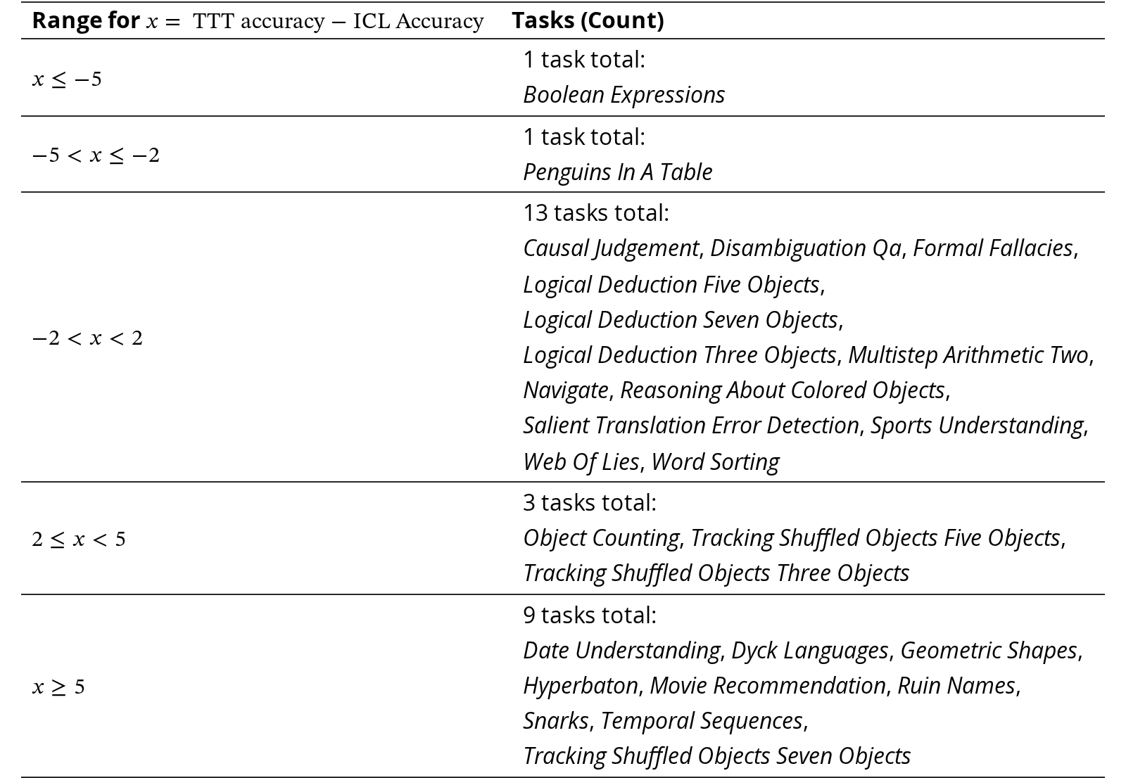
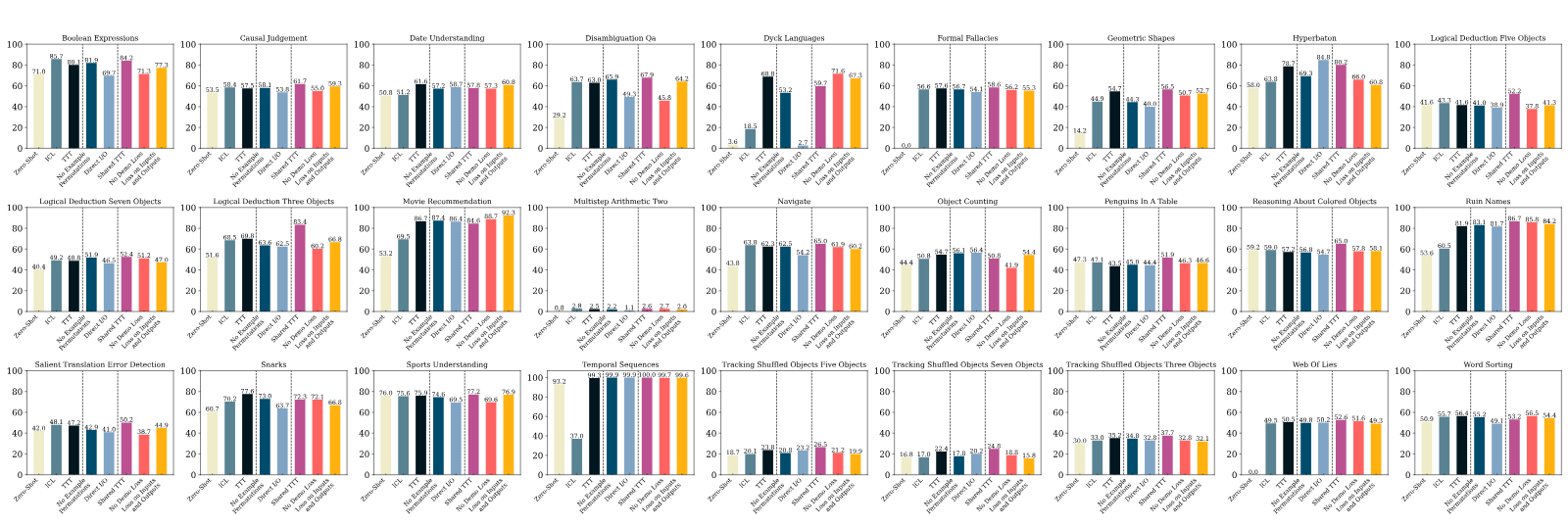
Our task-specific results show that performance improvements from TTT are highly task-dependent. Among the tasks in BBH, TTT results in a performance decline of at least compared to ICL in only tasks. In contrast, tasks show an improvement of at least , with of these showing improvements of at least . The four tasks with the most significant performance boost from TTT over ICL or zero-shot and the task with the most significant performance decrease are shown in Figure 9. These tasks in order of TTT’s improvement over ICL are Dyck Languages (parentheses matching), Ruin Names (humorous name modifications), Movie Recommendation (choosing similar films), Hyperbaton (adjective ordering), and Boolean Expression (evaluating a boolean expression). Detailed results for every task are given in Section F.2.
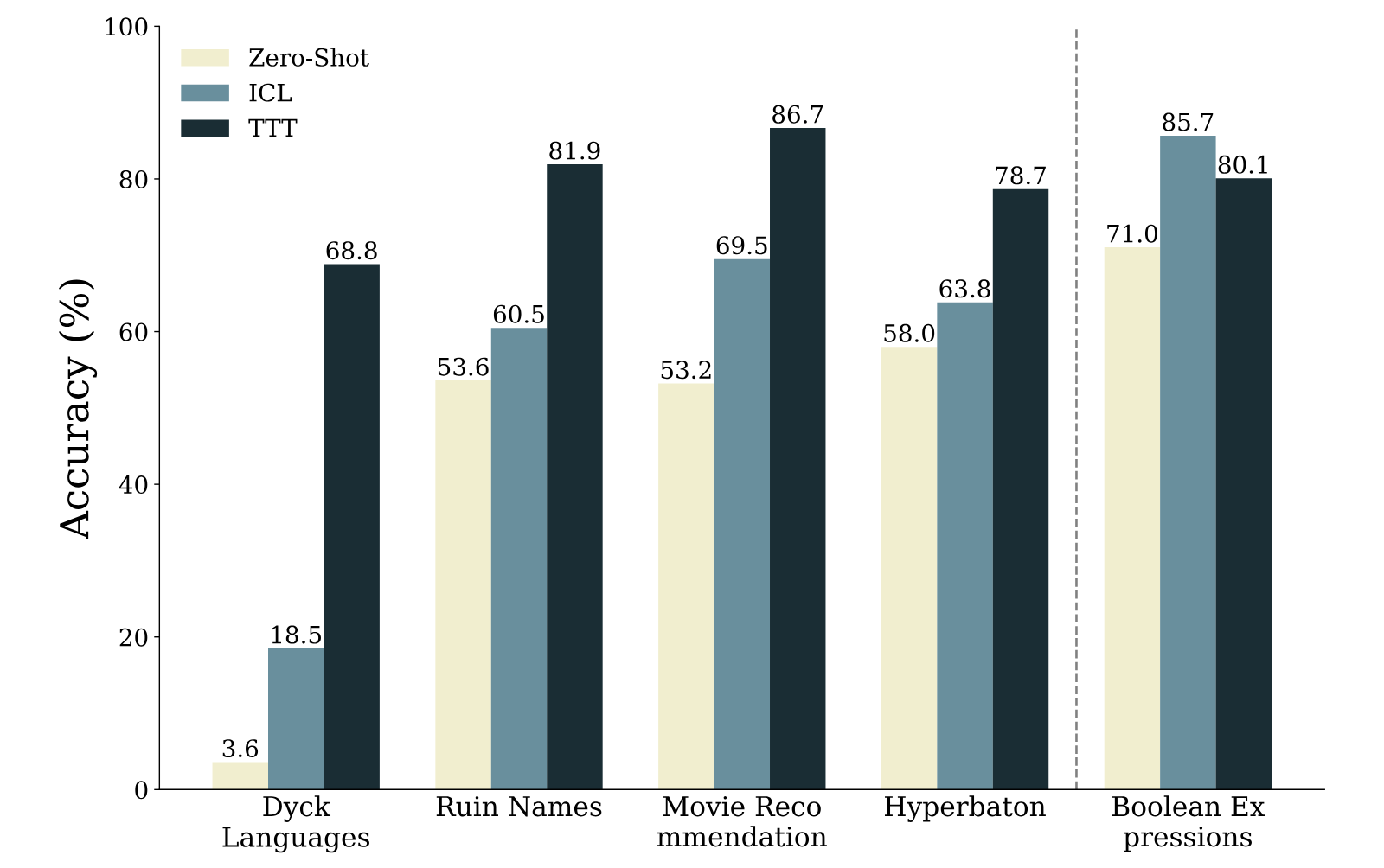
We hypothesize that improvements from TTT may be driven by tasks involving distribution shifts and structured patterns. For example, tasks like Dyck Languages and Hyperbaton follow clear grammatical or programmatic rules, which could align well with TTT’s ability to adapt to latent structural regularities during test-time.
Conversely, tasks requiring explicit step-by-step computation show limited gains with TTT. For instance, Boolean Expressions declined from to under TTT. This task’s algorithmic nature—dependent on sequential reasoning rather than pattern-based transduction—and its likely pre-training exposure suggest TTT’s updates may not resolve its specific demands. While these particular observations align with our hypothesis, the reason certain tasks benefit more from TTT remains an open question.
The idea of updating model parameters at test-time using instance-specific data traces back to early work on local learning (Bottou & Vapnik, 1992). More recently, Sun et al. (2020) propose a simple test-time self-supervision scheme to adapt an image classifier when facing distribution shifts. In language modeling, Hardt & Sun (2024) fine-tune on retrieved neighbors at test-time for notable gains, while Hübotter et al. (2025) optimize retrieval via active data selection.
Abstraction and Reasoning Corpus (Chollet, 2019; Chollet et al., 2025, ARC;) is a collection of extremely challenging few-shot visual reasoning problems. Most approaches to ARC fall into two main categories: program synthesis and fully neural. Program synthesis approaches (Butt et al., 2024; Wang et al., 2024; Li et al., 2025; Greenblatt, 2024) first try to find the transformation function , and then apply it to the test example. Fully neural approaches (Veldkamp et al., 2023; Bober-Irizar & Banerjee, 2024) try to directly predict the output , only implicitly modeling . In this work, we use a fully neural approach, using an LM to predict the test outputs. Recent work has explored hybrid methods, leveraging inference scaling and deep learning-guided program synthesis (Greenblatt, 2024; Li et al., 2025). Similarly, we find that integrating our neural model with program synthesis improves performance.
We conduct an investigation of test-time training and demonstrate that it can significantly improve LM performance on abstract reasoning and few-shot learning tasks, namely the Abstraction and Reasoning Corpus (ARC) and BIG-Bench Hard (BBH). Our key contributions include a robust TTT framework with leave-one-out in-context task construction, the optimization setup, and the inference strategy after TTT. Our results reveal the potential of TTT to tackle novel reasoning tasks, suggesting significant promise for test-time methods in advancing the next generation of LMs.
In development of ARC, we used a set of 80 tasks for validation/ablation experiments. Standard hyper-parameters (learning rate, epochs) were optimized using this set, which might have introduced some bias.
While the base Llama-3 performs poorly on the public validation set of ARC, the public availability of the dataset introduces the possibility that these models may have seen these examples during pre-training. Similarly, while the base model achieves reasonable performance on BBH, its public availability raises similar concerns.
We sincerely thank the BARC team (Li et al., 2025) for their support and collaboration in ensembling our method with theirs, resulting in an official joint submission to the ARC public set. We thank Aniruddha Nrusimha for helpful discussions on parameter efficient training. This work was supported by MIT–IBM Watson AI Lab, and by the National Science Foundation under grants IIS-2212310, IIS-2238240, and CCF-2217064. This work also benefited from many conversations during the Simons Institute Program on Language Models and Transformers.
References
- Acquaviva et al. (2022) Acquaviva, S., Pu, Y., Kryven, M., Sechopoulos, T., Wong, C., Ecanow, G. E., Nye, M. I., Tessler, M. H., and Tenenbaum, J. Communicating natural programs to humans and machines. In Advances in Neural Information Processing Systems 35, 2022. URL http://papers.nips.cc/paper_files/paper/2022/hash/182aed0379591ebd1d655b2bdc152075-Abstract-Datasets_and_Benchmarks.html.Source
- Akyürek et al. (2023) Akyürek, E., Schuurmans, D., Andreas, J., Ma, T., and Zhou, D. What learning algorithm is in-context learning? Investigations with linear models. In The Eleventh International Conference on Learning Representations, 2023. URL https://openreview.net/pdf?id=0g0X4H8yN4I.Source
- Behrouz et al. (2025) Behrouz, A., Zhong, P., and Mirrokni, V. Titans: Learning to memorize at test time, 2025. URL https://arxiv.org/abs/2501.00663.Source
- Bober-Irizar & Banerjee (2024) Bober-Irizar, M. and Banerjee, S. Neural networks for abstraction and reasoning. Scientific Reports, 2024. ISSN 2045-2322. doi: 10.1038/s41598-024-73582-7. URL https://doi.org/10.1038/s41598-024-73582-7.Source
- Bottou & Vapnik (1992) Bottou, L. and Vapnik, V. Local learning algorithms. Neural Computation, 1992. ISSN 0899-7667. doi: 10.1162/neco.1992.4.6.888. URL https://doi.org/10.1162/neco.1992.4.6.888.Source
- Brown et al. (2024) Brown, B., Juravsky, J., Ehrlich, R., Clark, R., Le, Q. V., Ré, C., and Mirhoseini, A. Large language monkeys: Scaling inference compute with repeated sampling, 2024. URL https://arxiv.org/abs/2407.21787.Source
- Brown et al. (2020) Brown, T. B., Mann, B., Ryder, N., Subbiah, M., Kaplan, J., Dhariwal, P., Neelakantan, A., Shyam, P., Sastry, G., Askell, A., Agarwal, S., Herbert-Voss, A., Krueger, G., Henighan, T., Child, R., Ramesh, A., Ziegler, D. M., Wu, J., Winter, C., Hesse, C., Chen, M., Sigler, E., Litwin, M., Gray, S., Chess, B., Clark, J., Berner, C., McCandlish, S., Radford, A., Sutskever, I., and Amodei, D. Language models are few-shot learners. In Advances in Neural Information Processing Systems 33, 2020. URL https://proceedings.neurips.cc/paper/2020/hash/1457c0d6bfcb4967418bfb8ac142f64a-Abstract.html.Source
- Butt et al. (2024) Butt, N., Manczak, B., Wiggers, A., Rainone, C., Zhang, D. W., Defferrard, M., and Cohen, T. CodeIt: Self-improving language models with prioritized hindsight replay. In Proceedings of the 41st International Conference on Machine Learning. PMLR, 2024. URL https://dl.acm.org/doi/10.5555/3692070.3692267.Source
- Chollet (2019) Chollet, F. On the measure of intelligence, 2019. URL https://arxiv.org/abs/1911.01547.Source
- Chollet et al. (2025) Chollet, F., Knoop, M., Kamradt, G., and Landers, B. ARC Prize 2024: Technical report, 2025. URL https://arxiv.org/abs/2412.04604.Source
- Damani et al. (2025) Damani, M., Shenfeld, I., Peng, A., Bobu, A., and Andreas, J. Learning how hard to think: Input-adaptive allocation of LM computation. In The Thirteenth International Conference on Learning Representations, 2025. URL https://openreview.net/forum?id=6qUUgw9bAZ.Source
- Dettmers et al. (2023) Dettmers, T., Pagnoni, A., Holtzman, A., and Zettlemoyer, L. QLoRA: Efficient finetuning of quantized LLMs. In Advances in Neural Information Processing Systems 36, 2023. URL http://papers.nips.cc/paper_files/paper/2023/hash/1feb87871436031bdc0f2beaa62a049b-Abstract-Conference.html.Source
- Gandelsman et al. (2022) Gandelsman, Y., Sun, Y., Chen, X., and Efros, A. A. Test-time training with masked autoencoders. In Advances in Neural Information Processing Systems 35, 2022. URL http://papers.nips.cc/paper_files/paper/2022/hash/bcdec1c2d60f94a93b6e36f937aa0530-Abstract-Conference.html.Source
- Greenblatt (2024) Greenblatt, R. Getting 50% (SoTA) on ARC-AGI with GPT-4o, 2024. URL https://redwoodresearch.substack.com/p/getting-50-sota-on-arc-agi-with-gpt. Accessed 09-11-2024.Source
- Hardt & Sun (2024) Hardt, M. and Sun, Y. Test-time training on nearest neighbors for large language models. In The Twelfth International Conference on Learning Representations, 2024. URL https://openreview.net/forum?id=CNL2bku4ra.Source
- Hodel (2024) Hodel, M. Addressing the Abstraction and Reasoning Corpus via procedural example generation, 2024. URL https://arxiv.org/abs/2404.07353.Source
- Hu et al. (2022) Hu, E. J., Shen, Y., Wallis, P., Allen-Zhu, Z., Li, Y., Wang, S., Wang, L., and Chen, W. LoRA: Low-rank adaptation of large language models. In The Tenth International Conference on Learning Representations, 2022. URL https://openreview.net/forum?id=nZeVKeeFYf9.Source
- Hübotter et al. (2025) Hübotter, J., Bongni, S., Hakimi, I., and Krause, A. Efficiently learning at test-time: Active fine-tuning of LLMs. In The Thirteenth International Conference on Learning Representations, 2025. URL https://openreview.net/forum?id=NS1G1Uhny3.Source
- Hurst et al. (2024) Hurst, A., Lerer, A., Goucher, A. P., Perelman, A., Ramesh, A., Clark, A., Ostrow, A., Welihinda, A., Hayes, A., Radford, A., et al. GPT-4o system card. ArXiv preprint, 2024. URL https://arxiv.org/abs/2410.21276.Source
- Joachims (1999) Joachims, T. Transductive inference for text classification using support vector machines. In Proceedings of the 16th International Conference on Machine Learning. Morgan Kaufmann Publishers Inc., 1999. ISBN 1558606122.
- Kwon et al. (2023) Kwon, W., Li, Z., Zhuang, S., Sheng, Y., Zheng, L., Yu, C. H., Gonzalez, J., Zhang, H., and Stoica, I. Efficient memory management for large language model serving with PagedAttention. In Proceedings of the 29th Symposium on Operating Systems Principles, SOSP ’23. Association for Computing Machinery, 2023. ISBN 9798400702297. doi: 10.1145/3600006.3613165. URL https://doi.org/10.1145/3600006.3613165.Source
- LeGris et al. (2024) LeGris, S., Vong, W. K., Lake, B. M., and Gureckis, T. M. H-ARC: A robust estimate of human performance on the Abstraction and Reasoning Corpus benchmark. ArXiv preprint, 2024. URL https://arxiv.org/abs/2409.01374.Source
- Li et al. (2025) Li, W.-D., Hu, K., Larsen, C., Wu, Y., Alford, S., Woo, C., Dunn, S. M., Tang, H., Zheng, W.-L., Pu, Y., and Ellis, K. Combining induction and transduction for abstract reasoning. In The Thirteenth International Conference on Learning Representations, 2025. URL https://openreview.net/forum?id=UmdotAAVDe.Source
- Llama Team (2024) Llama Team. The Llama 3 herd of models, 2024. URL https://arxiv.org/abs/2407.21783.Source
- Loshchilov & Hutter (2018) Loshchilov, I. and Hutter, F. Fixing weight decay regularization in Adam, 2018. URL https://openreview.net/forum?id=rk6qdGgCZ.Source
- McCoy et al. (2024) McCoy, R. T., Yao, S., Friedman, D., Hardy, M. D., and Griffiths, T. L. Embers of autoregression show how large language models are shaped by the problem they are trained to solve. Proceedings of the National Academy of Sciences, 2024. doi: 10.1073/pnas.2322420121. URL https://www.pnas.org/doi/abs/10.1073/pnas.2322420121.Source
- Min et al. (2022a) Min, S., Lewis, M., Zettlemoyer, L., and Hajishirzi, H. MetaICL: Learning to learn in context. In Proceedings of the 2022 Conference of the North American Chapter of the Association for Computational Linguistics: Human Language Technologies. Association for Computational Linguistics, 2022a. doi: 10.18653/v1/2022.naacl-main.201. URL https://aclanthology.org/2022.naacl-main.201.Source
- Min et al. (2022b) Min, S., Lyu, X., Holtzman, A., Artetxe, M., Lewis, M., Hajishirzi, H., and Zettlemoyer, L. Rethinking the role of demonstrations: What makes in-context learning work? In Proceedings of the 2022 Conference on Empirical Methods in Natural Language Processing. Association for Computational Linguistics, 2022b. doi: 10.18653/v1/2022.emnlp-main.759. URL https://aclanthology.org/2022.emnlp-main.759.Source
- OpenAI (2024) OpenAI. GPT-4 technical report, 2024. URL https://arxiv.org/abs/2303.08774.Source
- Opiełka et al. (2024) Opiełka, G., Rosenbusch, H., Vijverberg, V., and Stevenson, C. E. Do large language models solve ARC visual analogies like people do?, 2024. URL https://arxiv.org/abs/2403.09734.Source
- Ravi & Larochelle (2017) Ravi, S. and Larochelle, H. Optimization as a model for few-shot learning. In The Fifth International Conference on Learning Representations, 2017. URL https://openreview.net/forum?id=rJY0-Kcll.Source
- Snell et al. (2025) Snell, C. V., Lee, J., Xu, K., and Kumar, A. Scaling test-time compute optimally can be more effective than scaling LLM parameters. In The Thirteenth International Conference on Learning Representations, 2025. URL https://openreview.net/forum?id=4FWAwZtd2n.Source
- Srivastava et al. (2023) Srivastava, A., Rastogi, A., Rao, A., Shoeb, A. A. M., Abid, A., Fisch, A., Brown, A. R., Santoro, A., Gupta, A., Garriga-Alonso, A., et al. Beyond the imitation game: Quantifying and extrapolating the capabilities of language models. Transactions on Machine Learning Research, 2023. ISSN 2835-8856. URL https://openreview.net/forum?id=uyTL5Bvosj.Source
- Sun et al. (2020) Sun, Y., Wang, X., Liu, Z., Miller, J., Efros, A. A., and Hardt, M. Test-time training with self-supervision for generalization under distribution shifts. In Proceedings of the 37th International Conference on Machine Learning. PMLR, 2020. URL http://proceedings.mlr.press/v119/sun20b.html.Source
- Sun et al. (2024) Sun, Y., Li, X., Dalal, K., Xu, J., Vikram, A., Zhang, G., Dubois, Y., Chen, X., Wang, X., Koyejo, S., Hashimoto, T., and Guestrin, C. Learning to (learn at test time): RNNs with expressive hidden states, 2024. URL https://arxiv.org/abs/2407.04620.Source
- Suzgun et al. (2023) Suzgun, M., Scales, N., Schärli, N., Gehrmann, S., Tay, Y., Chung, H. W., Chowdhery, A., Le, Q., Chi, E., Zhou, D., and Wei, J. Challenging BIG-Bench tasks and whether chain-of-thought can solve them. In Findings of the 2023 Conference of the Association for Computational Linguistics. Association for Computational Linguistics, 2023. doi: 10.18653/v1/2023.findings-acl.824. URL https://aclanthology.org/2023.findings-acl.824.Source
- Todd et al. (2024) Todd, E., Li, M., Sharma, A. S., Mueller, A., Wallace, B. C., and Bau, D. Function vectors in large language models. In The Twelfth International Conference on Learning Representations, 2024. URL https://openreview.net/forum?id=AwyxtyMwaG.Source
- torchtune Maintainers & Contributors (2024) torchtune Maintainers and Contributors. torchtune: PyTorch’s finetuning library, 2024. URL https://github.com/pytorch/torchtune.Source
- Veldkamp et al. (2023) Veldkamp, K., Rosenbusch, H., Thoms, L., and Stevenson, C. Solving ARC visual analogies with neural embeddings and vector arithmetic: A generalized method. OSF, 2023. doi: 10.17605/OSF.IO/AKP86. URL https://osf.io/akp86/.Source
- Wang et al. (2025) Wang, K. A., Shi, J., and Fox, E. B. Test-time regression: a unifying framework for designing sequence models with associative memory. ArXiv preprint, 2025. URL https://arxiv.org/abs/2501.12352.Source
- Wang et al. (2024) Wang, R., Zelikman, E., Poesia, G., Pu, Y., Haber, N., and Goodman, N. Hypothesis Search: Inductive reasoning with language models. In The Twelfth International Conference on Learning Representations, 2024. URL https://openreview.net/forum?id=G7UtIGQmjm.Source
- Wang et al. (2023) Wang, X., Wei, J., Schuurmans, D., Le, Q. V., Chi, E. H., Narang, S., Chowdhery, A., and Zhou, D. Self-consistency improves chain of thought reasoning in language models. In The Eleventh International Conference on Learning Representations, 2023. URL https://openreview.net/forum?id=1PL1NIMMrw.Source
- Wei et al. (2022) Wei, J., Wang, X., Schuurmans, D., Bosma, M., Ichter, B., Xia, F., Chi, E. H., Le, Q. V., and Zhou, D. Chain-of-thought prompting elicits reasoning in large language models. In Advances in Neural Information Processing Systems 35, 2022. URL http://papers.nips.cc/paper_files/paper/2022/hash/9d5609613524ecf4f15af0f7b31abca4-Abstract-Conference.html.Source
- Wu et al. (2024) Wu, Z., Qiu, L., Ross, A., Akyürek, E., Chen, B., Wang, B., Kim, N., Andreas, J., and Kim, Y. Reasoning or reciting? Exploring the capabilities and limitations of language models through counterfactual tasks. In Proceedings of the 2024 Conference of the North American Chapter of the Association for Computational Linguistics: Human Language Technologies. Association for Computational Linguistics, 2024. URL https://aclanthology.org/2024.naacl-long.102.Source
- Yao et al. (2023) Yao, S., Yu, D., Zhao, J., Shafran, I., Griffiths, T., Cao, Y., and Narasimhan, K. Tree of Thoughts: Deliberate problem solving with large language models. In Advances in Neural Information Processing Systems 36, 2023. URL http://papers.nips.cc/paper_files/paper/2023/hash/271db9922b8d1f4dd7aaef84ed5ac703-Abstract-Conference.html.Source
- Zhao et al. (2024) Zhao, S., Nguyen, T., and Grover, A. Probing the decision boundaries of in-context learning in large language models. In ICML 2024 Workshop on In-Context Learning, 2024. URL https://openreview.net/forum?id=rfCtCcPuSt.Source
We present the tasks in the development set, the data format and evaluation details for the ARC dataset (available at this https link.).
We use numpy’s array printing format for all experiments as shown in Figure 10.
We use the following (Table 2) tasks validation tasks for our development.
| ID | Level | ID | Level | ID | Level | ID | Level |
|---|---|---|---|---|---|---|---|
| 0a1d4ef5 | easy | 762cd429 | medium | e5c44e8f | hard | e99362f0 | expert |
| 692cd3b6 | easy | e7639916 | medium | 604001fa | hard | 1acc24af | expert |
| 1da012fc | easy | e1d2900e | medium | 4364c1c4 | hard | f9a67cb5 | expert |
| 66e6c45b | easy | aee291af | medium | 506d28a5 | hard | ad7e01d0 | expert |
| 3194b014 | easy | e95e3d8e | medium | 2037f2c7 | hard | ea9794b1 | expert |
| 963f59bc | easy | e0fb7511 | medium | d5c634a2 | hard | 58e15b12 | expert |
| d37a1ef5 | easy | ae58858e | medium | ac605cbb | hard | 891232d6 | expert |
| 358ba94e | easy | 93c31fbe | medium | 27f8ce4f | hard | 5833af48 | expert |
| f3cdc58f | easy | 27a77e38 | medium | 66f2d22f | hard | 4ff4c9da | expert |
| 55059096 | easy | 9bebae7a | medium | 3ed85e70 | hard | 5b692c0f | expert |
| c7d4e6ad | easy | 9ddd00f0 | medium | 8b28cd80 | hard | e2092e0c | expert |
| 4b6b68e5 | easy | fe9372f3 | medium | d19f7514 | hard | 47996f11 | expert |
| 00576224 | easy | 69889d6e | medium | dc2aa30b | hard | 34b99a2b | expert |
| a04b2602 | easy | 15663ba9 | medium | f5c89df1 | hard | 1c56ad9f | expert |
| e9c9d9a1 | easy | 17b80ad2 | medium | 50f325b5 | hard | e6de6e8f | expert |
| ef26cbf6 | easy | 16b78196 | medium | 08573cc6 | hard | fea12743 | expert |
| 7ee1c6ea | easy | 5b6cbef5 | medium | 3d31c5b3 | hard | 31d5ba1a | expert |
| e9ac8c9e | easy | 40f6cd08 | medium | 94133066 | hard | 79fb03f4 | expert |
| 1a2e2828 | easy | 505fff84 | medium | 136b0064 | hard | 8719f442 | expert |
| 770cc55f | easy | d017b73f | medium | 90347967 | hard | a8610ef7 | expert |
View original table
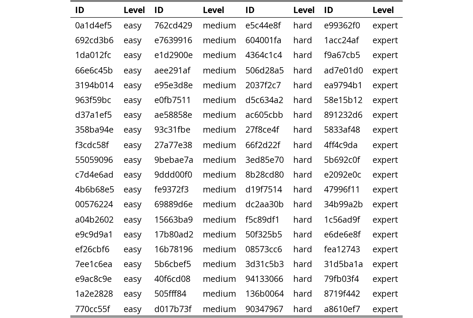
We follow the competition rules that if any of the two pass@2 predictions of the system is correct, we consider that test correct. In the reported task-level accuracies, we did not give partial points if all tests are not solved, except the final table Table 1.

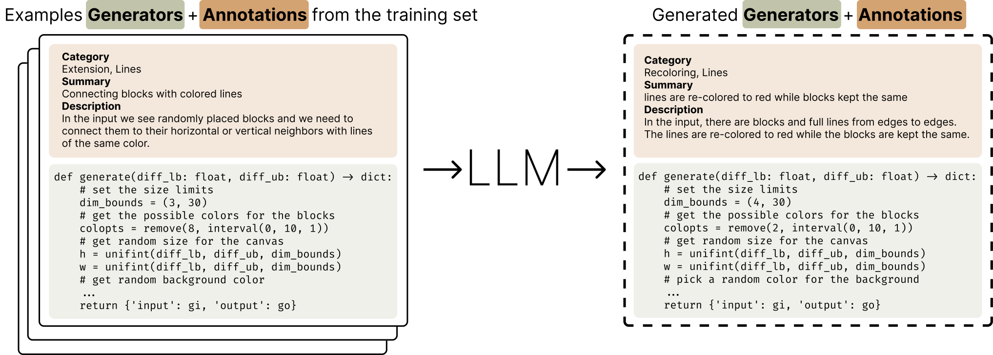
While test-time training facilitates task-specific adaptation, the base model’s capabilities impacts the final performance. We developed several approaches for generating synthetic training data to enhance the base model’s abstract reasoning capabilities through fine-tuning, exploring both automated and semi-automated methods for task generation. In this section, we detail our fine-tuning data generation strategies and analyze the impact of different data sources and model sizes on final performance.
(Hodel, 2024) provides domain-specific language (DSL), ReARC, as well as the transformation that solves the task-, and the data generation function that are implemented in this DSL for each training task in the dataset. These functions enable sampling of new input-output pairs that maintains the same underlying transformation principle:
where represents a newly generated input-output pair that can be solved using the same transformation function as the original task- .
The generator functions in ReARC already provide an effective data augmentation tool by producing different instantiations of same tasks. We generate extra samples from these training tasks by running the code many times and randomly splitting these new examples () to a set of train and test examples. These augmented examples are already provided with their DSL release.
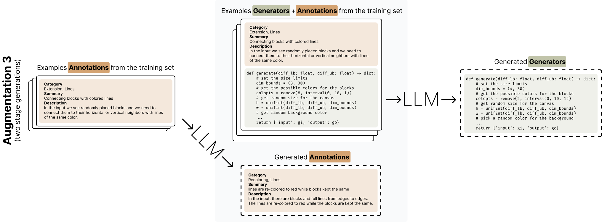
Additionally, we used several approaches to generate novel tasks using an LM (in our case, an ensemble of GPT4 and GPT4-o).
The simplest approach generates new task generators using few-shot examples:
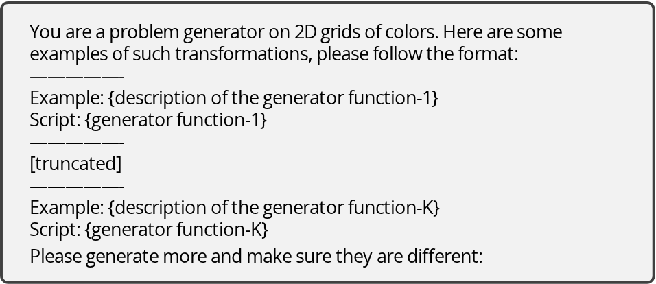
where is a new generator function and are existing generator functions (shown in Figure 11). We sample different examples by uniformly from existing training set. We repeat this process multiple times to get a good amount of tasks.
We augment the generator functions with task descriptions and jointly generate both descriptions and generators:
where represents the description of task .
To get the task descriptions, we manually created seed descriptions for training tasks. These seed descriptions were then used to generate descriptions for the training and validation tasks through few-shot prompting. To increase diversity of tasks, we use task descriptions with hierarchical fields (category, summary, and description). The process of getting these descriptions is provided in Section D.1.
Instead of jointly generating task descriptions and function generations, we additionally deployed a two-stage approach (Figure 12 ) described as following:
This approach first generates a task description and then conditions the generator creation on both existing task pairs and the new description. In total we collected 6426 generators with these LLM based approaches. We provide qualitative samples from these LM generated tasks in Figure 16.
Finally, our synthetic tasks are enhanced through various geometric transformations, such as basic transformations (rotations, reflections, random shift and size scaling), pattern operations (random patching, tiling, and repetition), color permutations, and composite transformations involving sequential application of multiple basic transformations. These transformations are applied in three ways:
- •
Input grids only:
- •
Output grids only:
- •
Both input and output:
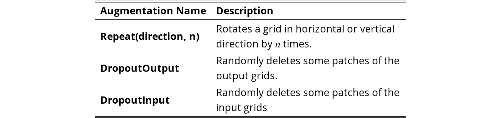
We use all the transformations given in Section C.1, and some additional transformations given in Table 3. In the fine-tuning case, different from TTT, we apply augmentations to only inputs, only outputs or both. These transformations are applied randomly to variants of tasks with of the time.
| Augmentation Name | Description |
|---|---|
| Repeat(direction, n) | Rotates a grid in horizontal or vertical direction by times. |
| DropoutOutput | Randomly deletes some patches of the output grids. |
| DropoutInput | Randomly deletes some patches of the input grids |
View original table
We perform full fine-tuning on LLama-3 family models by using the torchtune library. We train each model up to 16000 steps. We use 2xNVIDIA A100 GPU for 1B models, 4xNVIDIA A100 GPU for 3B and 8B models. We present hyperparameters in Table 4.
| Hyperparameter | Search Space |
|---|---|
| learning rate | 2.5e-5 |
| epochs | 2 |
| batch size | 32 |
| optimizer | AdamW (Loshchilov & Hutter, 2018) |
| scheduler | Cosine LR Schedule with 2k warmup |
View original table

We perform full fine-tuning 1B, 3B Llama 3.2 instruction-tuned, and 8B Llama 3 instruction-tuned using augmented data. The format and training objective is same as the ones described for TTT in 3. Hyperparameter details are given in Section C.2. We do the following ablations for augmented data:
- 1.
No FT: The original Llama 3 instruction-tuned model without any fine-tuning.
- 2.
All: We use all methods described in Section B.1, including ReARC, rule-based augmentation, and LM generation.
- 3.
No-Geom: We remove geometric transformations from all tasks.
- 4.
No-LM: We only use ReARC and rule-based augmentation, excluding tasks generated by the LM.
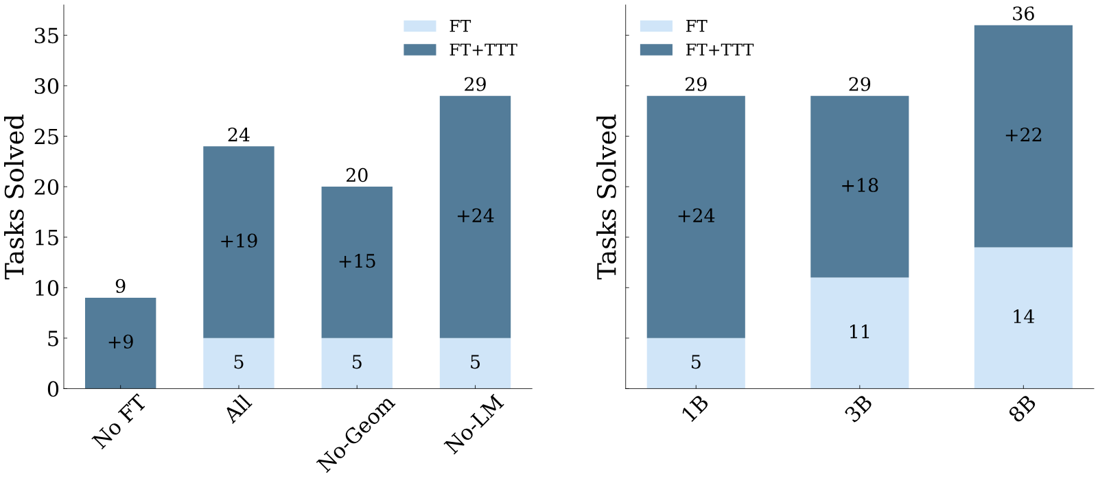
We show results using different model sizes in Figure 13. Increasing the model size consistently improves FT performance, with the 8B model achieving the highest accuracy of . We also observe that TTT effectively closes the performance gap for smaller models, with the 1B and 3B models achieving similar accuracy after TTT.
We present the transformations used in TTT and the training details.
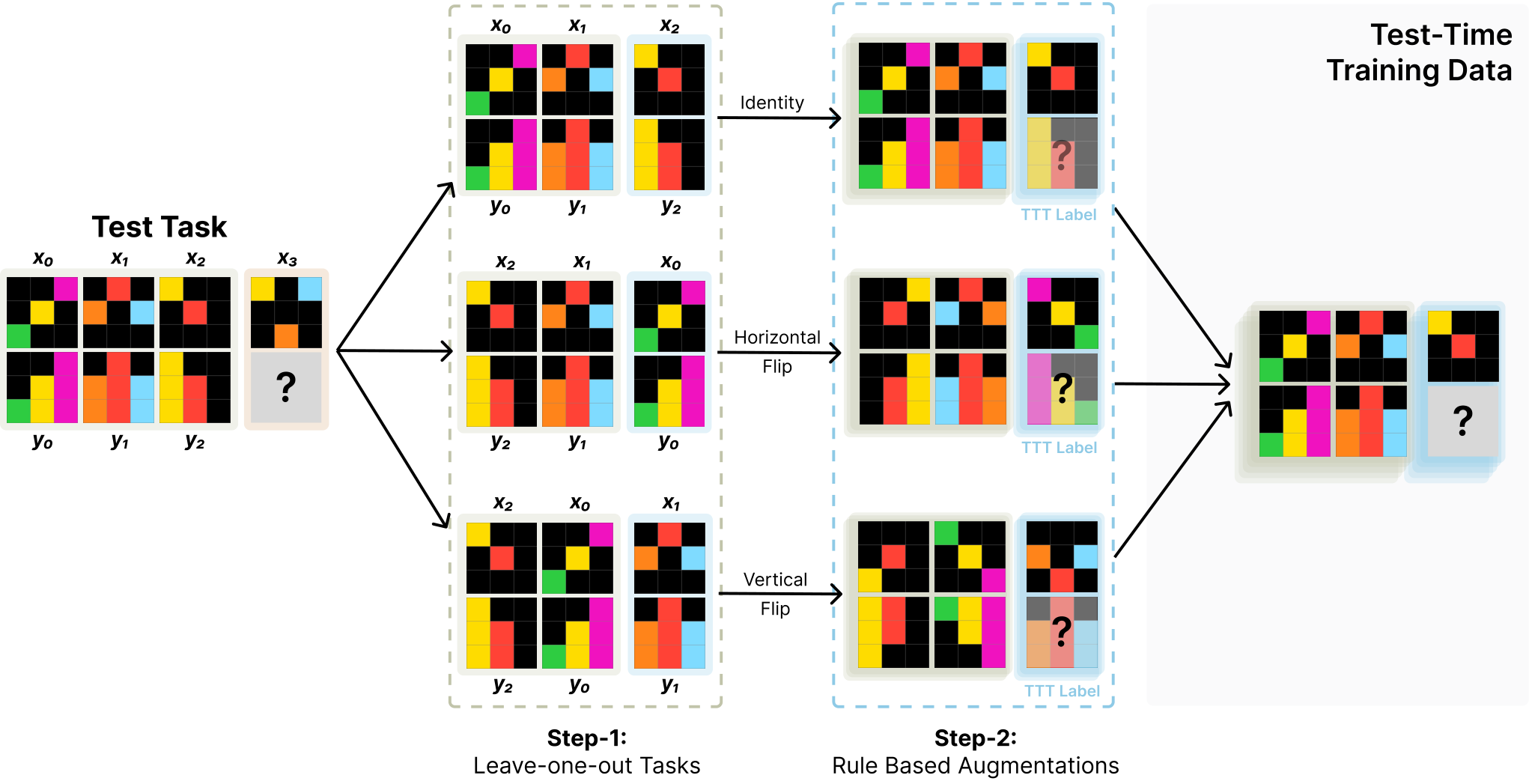
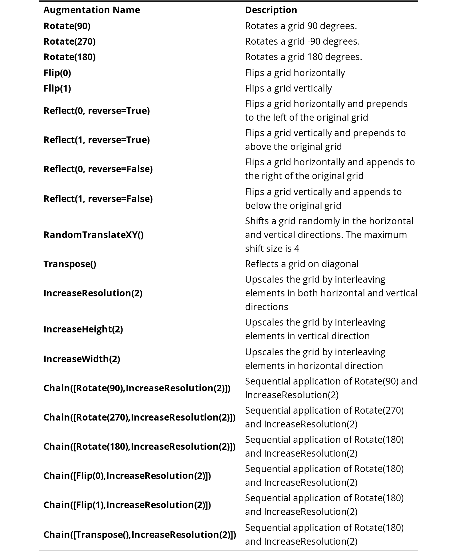
We provide the augmentations used in TTT in Table 5, please refer to our code base for their implementations. After applying these augmentations, we additionally shuffle colors and shuffle training examples. Note that these transformations are applied to all input and output grids. The procedure for generating the dataset for TTT is shown in Figure 14.
| Augmentation Name | Description |
|---|---|
| Rotate(90) | Rotates a grid 90 degrees. |
| Rotate(270) | Rotates a grid -90 degrees. |
| Rotate(180) | Rotates a grid 180 degrees. |
| Flip(0) | Flips a grid horizontally |
| Flip(1) | Flips a grid vertically |
| Reflect(0, reverse=True) | Flips a grid horizontally and prepends to the left of the original grid |
| Reflect(1, reverse=True) | Flips a grid vertically and prepends to above the original grid |
| Reflect(0, reverse=False) | Flips a grid horizontally and appends to the right of the original grid |
| Reflect(1, reverse=False) | Flips a grid vertically and appends to below the original grid |
| RandomTranslateXY() | Shifts a grid randomly in the horizontal and vertical directions. The maximum shift size is 4 |
| Transpose() | Reflects a grid on diagonal |
| IncreaseResolution(2) | Upscales the grid by interleaving elements in both horizontal and vertical directions |
| IncreaseHeight(2) | Upscales the grid by interleaving elements in vertical direction |
| IncreaseWidth(2) | Upscales the grid by interleaving elements in horizontal direction |
| Chain([Rotate(90),IncreaseResolution(2)]) | Sequential application of Rotate(90) and IncreaseResolution(2) |
| Chain([Rotate(270),IncreaseResolution(2)]) | Sequential application of Rotate(270) and IncreaseResolution(2) |
| Chain([Rotate(180),IncreaseResolution(2)]) | Sequential application of Rotate(180) and IncreaseResolution(2) |
| Chain([Flip(0),IncreaseResolution(2)]) | Sequential application of Rotate(180) and IncreaseResolution(2) |
| Chain([Flip(1),IncreaseResolution(2)]) | Sequential application of Rotate(180) and IncreaseResolution(2) |
| Chain([Transpose(),IncreaseResolution(2)]) | Sequential application of Rotate(180) and IncreaseResolution(2) |
View original table
We use the torchtune(torchtune Maintainers & Contributors, 2024) library to train LoRA adapters on Llama-3 family of models. We apply LoRA training to query and value projection weights of the self-attention layer, to the MLP weights and to the output projection layer (was only available for Llama-3 8B in torchtune). We present hyperparameters of this training in Table 6. We also found that using quantized LoRA adapters (Dettmers et al., 2023) instead of standard (full-precision) LoRA leads to only a small drop in performance ( tasks solved with the 1B-parameter model), making it a viable option in memory-constrained settings.
We resort to the vLLM (Kwon et al., 2023) library for prediction as it provides fast kernels and batched inference for our models and LoRA inference. We just use greed decoding as we did not see improvements with temperature sampling in our early experiments. We use 90, 180 degree rotations, horizontal, vertical, and diagonal (transpose) flips as our invertible transformations.
With that, the whole TTT and inference process takes approximately hours for randomly sampled validation tasks when using an NVIDIA A100 GPU.
| Hyperparameter | Search Space |
|---|---|
| LoRA rank | 128 |
| LoRA alpha | 16 |
| learning rate | [5e-5, 1e-4] |
| epochs | 2 |
| batch size | [1, 2] |
| optimizer | AdamW (Loshchilov & Hutter, 2018) |
View original table

We described three approaches in Appendix B to use LM, we generated 6426 task generators by few-shot prompting GPT-4 and GPT-4o models (OpenAI, 2024; Hurst et al., 2024).
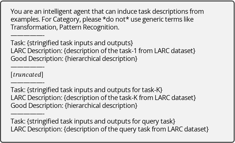
This procedure is shown in Figure 15. We initially described 10 training tasks with the hierarchical-style shown in Figure 11. Then, for other training tasks tasks, we obtained less quality crowd-worker annotations from LARC (Acquaviva et al., 2022) project. By using our high-quality seed annotations and their LARC version, we -shot prompt and LM to produce high quality annotations for the other training tasks.
Text in this graphic
You are an intelligent agent that can induce task descriptions from examples. For Category, please *do not* use generic terms like Transformation, Pattern Recognition.
—————-
Task: {stringified task inputs and outputs}
LARC Description: {description of the task-1 from LARC dataset}
Good Description: {hierarchical description}
—————-
—————-
Task: {stringified task inputs and outputs for task-K}
LARC Description: {description of the task-K from LARC dataset}
Good Description: {hierarchical description}
—————-
Task: {stringified task inputs and outputs for query task}
LARC Description: {description of the query task from LARC dataset}
We use the following simple prompting template with k-shot prompting for all data generation procedures, where numbers filled with examples sampled from seed set. In simple few-shot generation, we exclude examples. We use GPT-4 and GPT-4o to generate the new scripts.
Text in this graphic
You are a problem generator on 2D grids of colors. Here are some examples of such transformations, please follow the format:
—————-
Example: {description of the generator function-1}
Script: {generator function-1}
—————-
[truncated]
—————-
Example: {description of the generator function-K}
Script: {generator function-K}
Please generate more and make sure they are different:

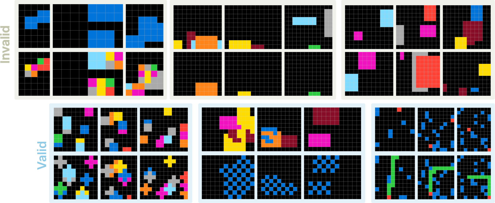
Recent work has shown that scaling test-time compute can significantly improve the performance of LMs. One of the most common techniques to do this is by sampling multiple responses, and then selecting the best response using a ranker. However, while sampling is very effective in domains with multiple possible solutions (programs in code) or multiple possible paths to the final answer (math), it can be detrimental when generating answers directly, as there is no way to directly enforce diversity across samples while ensuring coherence within samples. As an alternative inference-time scaling, we use an augmented inference strategy that generates multiple prediction candidates by using geometric transformations, combined with a greedy decoding scheme.
For a given task with training examples and test input , we use invertible geometric transformations to produce equivalent transformed versions of the task, as shown in Figure 5. Let be some set set of invertible geometric transformations (e.g., rotations and reflections). For each transformation , we apply to all training demonstrations and the test input and run our model with these transformed inputs. We then apply the inverse transformation to obtain the final prediction for that transformation.
We further augment our predictions by permuting the order of training examples. For each transformation , we sample different permutations of the demonstration sequence, resulting in total predictions per task. This is to mitigate any bias in the model’s processing of the demonstration sequence. (Bober-Irizar & Banerjee, 2024) also find transpose and rotation is helpful to produce extra prediction candidates.
We employ a hierarchical voting strategy to determine the final prediction from the set of candidates . This approach involves two stages of voting to progressively narrow down the best candidates: first, by selecting the most frequent predictions within each transformation, and then by conducting an overall vote across transformation-specific candidates to identify the top-2 most frequent predictions. The details of each stage are as follows:
- 1.
Intra Transformation Voting: We group predictions by their corresponding transformation and select the top-3 most frequent predictions within each group. If fewer than 3 unique predictions exist within a group, we supplement the candidates by computing additional predictions through:
- •
Row-based majority: For each row in the predicted output grid, we take the most frequent row values across all predictions in the transformation group.
- •
Column-based majority: Similarly, for each column in the predicted output grid, we take the most frequent column values across all predictions in the transformation group.
- •
- 2.
Global Voting: Using the selected transformation-specific candidates obtained from (1), we conduct an overall vote to select the top-2 most frequent predictions for submission. In case of a tie, predictions with the identity transformation are given priority.
We write our own evaluation function for BIG-Bench Hard available in our codebase. We found that existing evaluation frameworks did not properly measure zero-shot performance due to insufficient answer-extraction parsing and answer-format prompting. We also wanted more control in splitting each individual task’s dataset into demonstration examples and evaluation sets. For all results, we average results over different selections of the few-shot examples with the following random seeds: . The full TTT and inference process takes approximately 15 minutes on an NVIDIA A100 GPU.
| Method | Standard Error of the Mean |
|---|---|
| Zero-Shot | 0.01 |
| ICL | 0.19 |
| TTT | 0.20 |
| No Example Permutation | 0.32 |
| E2E | 0.66 |
| Shared TTT | 0.72 |
| No Demo Loss | 0.69 |
| Loss on Inputs and Outputs | 0.35 |
View original table
We search over the following hyperparameters:
| Hyperparameter | Search Space |
|---|---|
| learning rate | [1e-5, 5e-5, 1e-4, 3e-4] |
| LoRA rank | [64, 128] |
| LoRA alpha | [16, 32, 64, 128] |
| epochs | 1 |
| batch size | 5 |
| training steps | [20, 40, 60] |
| optimizer | AdamW |
| scheduler | Cosine LR Schedule |
View original table

We similarly use the torchtune(torchtune Maintainers & Contributors, 2024) library for test-time training and the vLLM (Kwon et al., 2023) library for inference.
The full results for all tasks over all methods and ablations are shown in Figure 17.
| Range for | Tasks (Count) |
|---|---|
| 1 task total: Boolean Expressions | |
| 1 task total: Penguins In A Table | |
| 13 tasks total: Causal Judgement, Disambiguation Qa, Formal Fallacies, Logical Deduction Five Objects, Logical Deduction Seven Objects, Logical Deduction Three Objects, Multistep Arithmetic Two, Navigate, Reasoning About Colored Objects, Salient Translation Error Detection, Sports Understanding, Web Of Lies, Word Sorting | |
| 3 tasks total: Object Counting, Tracking Shuffled Objects Five Objects, Tracking Shuffled Objects Three Objects | |
| 9 tasks total: Date Understanding, Dyck Languages, Geometric Shapes, Hyperbaton, Movie Recommendation, Ruin Names, Snarks, Temporal Sequences, Tracking Shuffled Objects Seven Objects |
View original table