Sundial: A Family of Highly Capable Time Series Foundation Models
arXiv:2502.00816v4 · This workspace stays on this version. Check arXiv for newer versions
Some source details need review 11 to check
Original formulas, table values and figures are preserved. Comparison can miss differences; use the original PDF to check details.
Reading view checked: 197 math expressions, 0 rendering failures; 24 of 24 images available.
Compared 116 of 116 source passages against 23 of 23 PDF pages.
- An unsupported comparison claim was rejected; source verification is incomplete.
- Additional source conflicts need review; automatic escalation was bounded to four.
HTML S1_p2_1 quotes “Liu et al., 2024a”; the original PDF page 1 quotes “Liu et al., 2024c”. Check PDF page 1
HTML block S2_SS2_p1_1 says “Liu et al., 2024b,” while the original PDF page 2 says “Liu et al., 2024a.” The PDF contradicts the HTML. Check PDF page 2
HTML [S2_SS2_p1_1] cites Timer as “Liu et al., 2024b” and “Liu et al., 2024c”; the original PDF (page 3) reads “Timer (Liu et al., 2024a;b).” Check PDF page 3
HTML S4_p1_1 says “Liu et al. (2024c)”; PDF page 4 says “Liu et al. (2024b)”, so the PDF contradicts the HTML. Check PDF page 4
The Liu et al. citation year differs. Check PDF page 9
The Liu et al. citation year differs. Check PDF page 13
The Liu et al. citation years differ. Check PDF page 13
The Liu et al. citation year differs. Check PDF page 13
The Liu et al. citation years differ. Check PDF page 16
24 of 24 figure, table and graphic images captured. Open original PDF
Abstract
We introduce Sundial, a family of native, flexible, and scalable time series foundation models. To predict the next-patch’s distribution, we propose a TimeFlow Loss based on flow-matching, which facilitates native pre-training of Transformers on continuous-valued time series without discrete tokenization. Conditioned on arbitrary-length time series, our models are pre-trained without specifying any prior distribution and can generate multiple probable predictions, achieving more flexibility in representation learning than using parametric densities. Towards time series foundation models, we leverage minimal but crucial adaptations of Transformers and curate TimeBench with one trillion time points, comprising mostly real-world datasets and synthetic data. By mitigating mode collapse via TimeFlow Loss, we pre-train a family of Sundial models on TimeBench, which achieve unprecedented model capacity and generalization performance. In addition to excellent scalability, Sundial achieves state-of-the-art results on both point and probabilistic forecasting benchmarks with a just-in-time inference speed, i.e., making zero-shot predictions within a few milliseconds. We believe that Sundial’s pioneering generative forecasting capability can improve model reliability in real-world decision-making. Code is available at: https://github.com/thuml/Sundial.
Time series forecasting has fascinated people for thousands of years. Although people have been able to determine the time using instruments like sundials in 3000 BC, time series forecasting is intrinsically non-deterministic (Box et al., 2015). Therefore, generating a variety of probable predictions is crucial for decision-making. The growing demand has facilitated numerous statistical approaches over the past decades (Hyndman, 2018; Box, 2013), which provide high-profile theories and probabilistic tools for making reliable schedules. Recent advancements bring the boom of deftly designed models that automatically learn intricate dynamics and correlations from raw data (Oreshkin et al., 2019; Nie et al., 2022; Zhang and Yan, 2023; Liu et al., 2023a). Despite the impressive performance, deep models necessitate task-specific training on sufficient in-distribution data. Motivated by advances in large models (Bommasani et al., 2021), pre-trained time series foundation models have shown promising capabilities in out-of-distribution tasks (Das et al., 2023b; Liu et al., 2024c; Woo et al., 2024; Ansari et al., 2024).
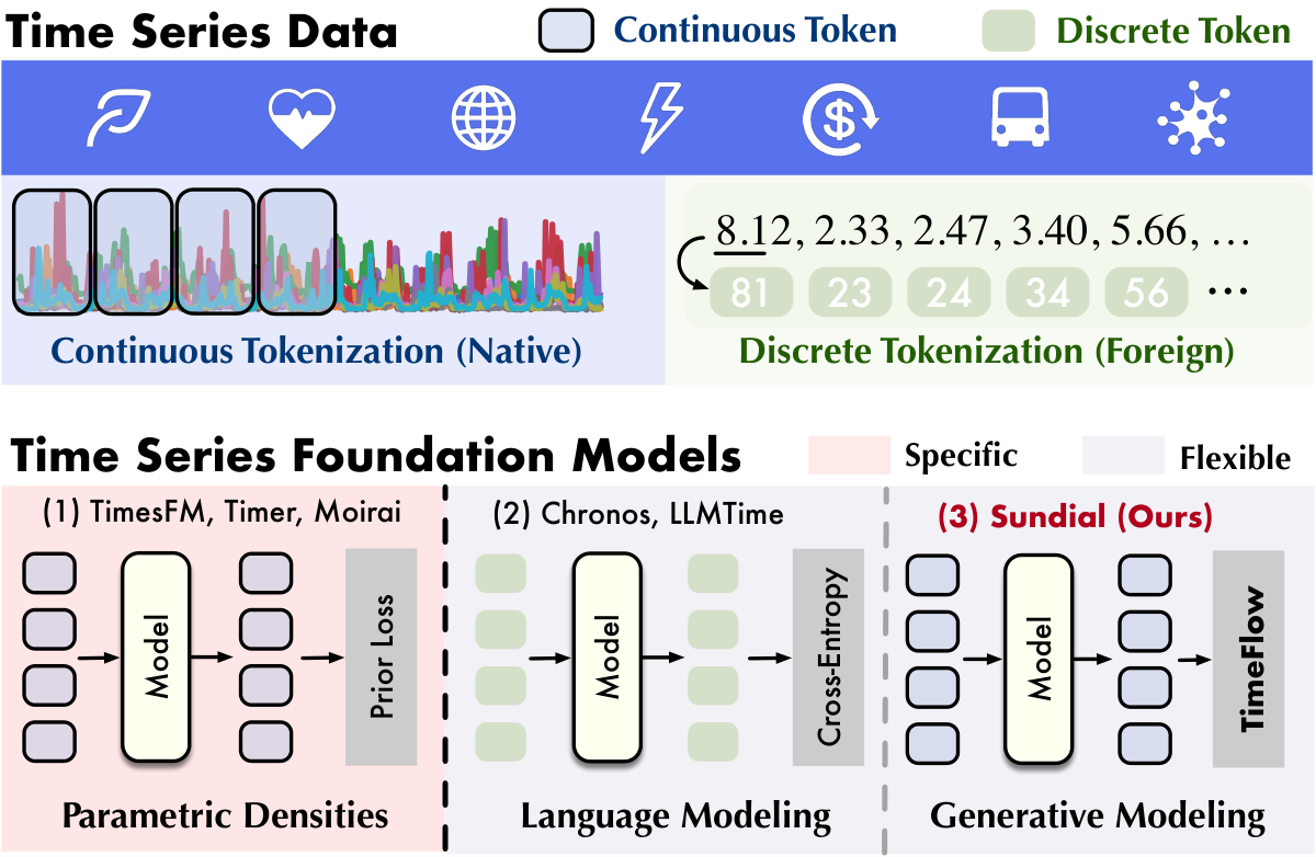
Current research on time series foundation models has converged on building unified, scalable, and out-of-the-box forecasters, exhibiting zero-shot performance close to or sometimes surpassing supervised methods (Aksu et al., 2024). Notably, Transformers (Radford et al., 2018) are currently the de facto architecture of these models. While pre-trained Transformers with an inherent generative ability have facilitated great success in language, image, and video generation (Ramesh et al., 2021; OpenAI, 2023; Liu et al., 2024a), most time series foundation models are not “generative” or, more specifically, probabilistic forecasters, thereby limiting reliability in decision-making. Although parametric densities specified with prior distributions (Wen et al., 2017; Woo et al., 2024) can be adopted to address uncertainty in time series forecasting, they can reduce the capacity of distributions learned by pre-trained models, especially on time series modality characterized by high heterogeneity. To learn arbitrarily intricate distributions without mode collapse, language modeling (Bengio et al., 2000) that learns the categorical distribution via cross-entropy loss inspires subsequent works (Gruver et al., 2023; Ansari et al., 2024), which treat time series as a foreign language using discrete tokenization. Still, discrepancies between continuous-valued time series and discrete language tokens can lead to out-of-vocabulary issues and coarse-grained prediction intervals.
As shown in Figure 1, Sundial is presented as the first family of generative models among time series foundation models. As foundation models intend to learn complicated distributions from extensive datasets and facilitate transferability across agnostic downstream datasets, we do not specify any prior parametric densities, such as unimodal and multimodal Gaussian mixtures. Instead, we delve into generative modeling to tame Transformers as native, flexible, and scalable time series foundation models. By comparing to denoising diffusion models (Li et al., 2024), we opt for a simple yet effective flow-matching framework (Lipman et al., 2022), which provides notable efficiency and sample quality (Tong et al., 2023). We propose TimeFlow Loss, a parameterized training objective (Zhang et al., 2018) for autoregressive models to learn and sample from each token’s predictive distribution. Optimizing models in the original continuous-valued domain, TimeFlow Loss facilitates patch-level generation and enables fast inference, which is naturally compatible with the time series modality.
In addition to TimeFlow, we enhance the Transformer with minimal but critical adaptations. We develop feasible patch tokenization for arbitrary-length input time series. We adopt RoPE (Su et al., 2024), Pre-LN (Xiong et al., 2020), FlashAttention (Dao et al., 2022), and KV Cache (Pope et al., 2023), which are crucial but generally neglected in the development of time series foundation models. Besides, we pre-train our models by multi-patch prediction to reduce autoregression steps. We realize a rapid generation of multiple samples by reusing a shared lookback representation. Beyond facilitating scalable pre-training, these adaptations help real-time long-context inference and long-term generation.
To validate the scaling law of time series foundation models, we collect and curate TimeBench with an unprecedented volume of a trillion time points. We present Sundial as a family of highly capable foundation models, which achieve state-of-the-art on three large-scale and best-recognized benchmarks, including Time-Series-Library (TSLib) (Wu et al., 2022), GIFT-Eval (Aksu et al., 2024), and FEV (Ansari et al., 2024). Our contributions lie in these aspects:
- •
We propose TimeFlow Loss to predict next-patch’s distribution, allowing Transformers to be trained without discrete tokenization and make probable predictions.
- •
We present Sundial, a family of scalable and efficient time series foundation models built upon our enhanced Transformer and pre-trained on a trillion time points.
- •
Experimentally, Sundial achieves state-of-the-art zero-shot performance on point and probabilistic forecasting benchmarks, including TSLib, GIFT-Eval, and FEV, indicating a promising generative approach for the future improvement of time series foundation models.
Forecasting is essential for decision-making. Advancements in deep learning for time series include theory-inspired deep modules (Wu et al., 2021; Liu et al., 2023b; Wu et al., 2022), architecture-oriented adaptations (Bai et al., 2018; Salinas et al., 2020; Lim et al., 2021), and time series preprocessing (Kim et al., 2021; Nie et al., 2022). Deep models learn the dataset-level distribution and benefit from strong generalization and model capacity. Statistical methods conduct case-by-case fitting on input series, achieving notable performance on small data (Ke et al., 2017; Hyndman, 2018).
One of the efforts towards more capable forecasters focuses on the foundation models (Bommasani et al., 2021), which address data-scarce scenarios by pre-training. More capable models support zero-shot forecasting, making inferences as fast as statistical methods and possessing large model capacity as deep models. Another aspect is to address uncertainty in time series forecasting. There is a growing research emphasis on probabilistic forecasting (Woo et al., 2024; Ansari et al., 2024). While parametric densities can be adopted as training objectives of probabilistic forecasting, they can be too specific to meet the heterogeneity of large-scale datasets, resulting in mode collapse in representation learning and over-smooth predictions (Figure 14-15). In this work, we introduce generative time series foundation models, which naturally address the uncertainty in forecasting.
Recent research has concentrated on building versatile large time series models (Liang et al., 2024). With the advances made in large language models, Transformer has become the dominant architecture. Several works adapt Transformers to address the unique 2D-dimensionality and heterogeneity of time series (Woo et al., 2024; Liu et al., 2024b). Specifically, our work delves into tokenization and optimization. Models such as TimesFM (Das et al., 2023b), Timer (Liu et al., 2024b; Liu et al., 2024c), and Time-MoE (Shi et al., 2024b) embed continuous values and fit unimodal distributions via MSE or quantile loss (Wen et al., 2017). However, prior loss may result in mode collapse because predictive distributions are highly divergent across different domains. Besides, these models cannot provide the confidence level of predictions, limiting reliability for decision-making. Based on continuous tokenization, Moirai (Woo et al., 2024) presents a probabilistic model learning a mixture of distributions, but this prior can still fail to accommodate complex distributions. Inspired by language modeling, Chronos (Ansari et al., 2024) discretizes series via bucket quantization, learning more flexible categorical distributions by cross-entropy. Still, discrete tokenization is applied at each time point, which can lead to long contexts. Also, the final performance can be sensitive to quantization techniques. Unlike before, we tame Transformers as native time series foundation models, learning flexible distributions without discrete tokenization.
By addressing complicated distributions during pre-training, generative modeling has become a focal point in the development of various foundation models (Zhao et al., 2023; Liu et al., 2024a). While this direction for time series mostly focused on time series generation (Tashiro et al., 2021) and task-specific forecasters (Rasul et al., 2021; Shen and Kwok, 2023; Kollovieh et al., 2024), generative modeling for time series foundation models is hardly explored. With the comparable flexibility in distribution learning as language modeling, diffusion denoising (Sohl-Dickstein et al., 2015) and flow-matching (Lipman et al., 2022) have gained increasing prevalence in continuous-valued modalities (Lipman et al., 2024). Compared with diffusion denoising models, flow-matching provides a simple yet efficient framework. With fewer steps involved in the forward and reverse processes, large models based on flow-matching have shown superior performance in image generation (Esser et al., 2024).
Despite the connection in value continuity, generating images and future time series are fundamentally different tasks due to the autoregressive property of forecasting. Our proposed TimeFlow Loss is designed for autoregressive models to conduct conditional generation, which is a parameterized loss function (Zhang et al., 2018) for arbitrary distributions and enhances representation learning of foundation models.
The goal of generative modeling is to learn the underlying probability distribution that generates the data. The framework of flow-matching transforms a sample drawn from a source distribution into a sample drawn from a target distribution. The transformation is continuous in time. For -dimensional distributions, it is defined by a time-dependent velocity field , which is the solution of the ordinary differential equation (ODE):
The velocity field determines a flow . For all , generates the probability path that interpolates and , i.e., for . The implementation of flow-matching is to train a network parametrized by to fit the velocity field , which is a regression-based task formulated as the Flow-Matching objective:
Furthermore, Lipman et al. (2022) proved the equivalence of optimizing the Conditional Flow-Matching objective:
Leveraging the conditional optimal-transport (linear) path and a source Gaussian, the objective can be formulated as:
where and .
Consequently, we can train a generative network on given samples from the target distribution, and generate new samples by applying a push-forward process on samples drawn from a simple source Gaussian distribution:
Given a historical observation , the target of time series forecasting is to predict future time series . The task can be generally formulated as , where is the learned representation from a deep model . In probabilistic forecasting, explicit optimization objectives are utilized to predict the statistics of future series, e.g., MSE or quantile loss, which have specified as a prior distribution. While using one parametric density generally fits well on a small amount of data, it can be the major bottleneck for scaling time series foundation models. Inspired by the success of large generative models (Rombach et al., 2022; OpenAI, 2023; Esser et al., 2024), we introduce generative modeling to realize probabilistic forecasting:
is a small trainable generative network conditioned on the learned representations of , which is jointly optimized with . While the generative model automatically fits the target distribution, it can sample raw predictions and calculating their statistics for probabilistic forecasting. The aim is conceptually related to conformal prediction (Vovk et al., 2005) but models uncertainty beyond prediction intervals.
In this work, we conduct a univariate pre-training paradigm, which adopts the S3 format proposed by Liu et al. (2024c) to address multivariate data. To mitigate value range discrepancy, we conduct normalization on time series individually per variable. Afterwards, we sample varying-length training samples with the maximum context length of . As a foundation model, Sundial is required to predict on out-of-distribution series with varied lengths during inference.
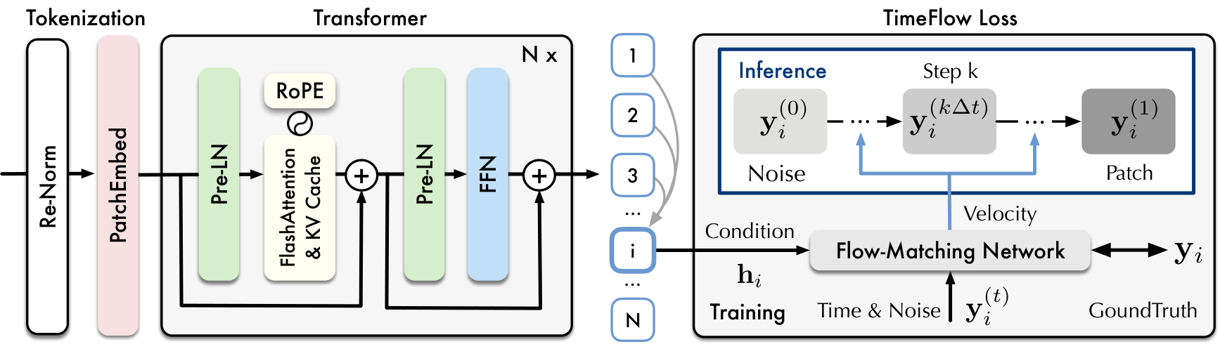
As shown in Figure 2, the Sundial models consist of three parts: (1) time series tokenization, including a context-level re-normalization and a patch embedding that addresses any-length time series, (2) a Transformer backbone that learns the per-token representation of time series, and (3) TimeFlow Loss, a parameterized loss function to model the per-token distribution and generate raw series during inference. Intuitively, Sundial can be regarded as an ARMA (Auto-Regression and Moving-Average) deep model, i.e., Transformer learns token representations autoregressively. Conditioned on the lookback representations, TimeFlow transforms random noises into non-deterministic predictions.
We adopt stationarization (Liu et al., 2022), a non-parametric two-stage instance normalization conducted within each sample, which is initially proposed to mitigate non-stationarity of time series. Here, it helps to address temporal distribution shift and outlier ranges in input series, improving generalizability for zero-shot forecasting.
Given a univariate time series , it is divided into patches with the length of . To address non-divisible length, we pad the input at the beginning and use a binary mask for each patch to indicate the padded position. It will lead to such input tokens. Subsequently, we use a shared MLP to embed all patch tokens:
where and is the dimension of token embedding. Unlike point-level quantization (Ansari et al., 2024), we reserve original values without discrete quantization. It also reduces the context length (in token) of the Transformer.
Given token embeddings , we adopt several crucial adaptations on a decoder-only Transformer to obtain per-token representations aggregated from all previous tokens. First, we adapt Pre-LN (Xiong et al., 2020) to improve pre-training stability. Second, we leverage a causal self-attention mechanism with RoPE (Su et al., 2024) that introduces the position information of patch tokens. It can be formulated as follows (the layer index is omitted for simplicity):
where project token embeddings into -dimensional queries, keys, and values. is the rotary matrix with rotation degree . Lastly, we implement FlashAttention (Dao et al., 2022) and KV Cache (Pope et al., 2023), since these enhancements for deployment are increasingly emphasized in large foundation models (Shoeybi et al., 2019; Rasley et al., 2020).
Given representations extracted by the last layer of the Transformer, we aim to generate length- predictions at each position via our autoregressive model. Motivated by the empirical observation that a larger patch size improves the performance in decoder-only Transformers (Das et al., 2023b) while a small patch size can be more flexible to accommodate data of different frequencies, we adopt multi-patch predictions () for pre-training, which also reduces the steps of autoregressive inference.
Based on Equations 1 and 3, we formulate a new generative forecasting conditioned on a sequential representation :
where is the groundtruth value and is a -dimensional Gaussian noise, is sampled from , and is constructed by the conditional optimal-transport path. It is important to note that the conditional representation differs from the conditional path and the conditional source distribution. Instead, is a condition of position , also a time-invariant condition of the whole flow-matching process . Technically, we implement the flow-matching network by a small MLP:
The training process involves sampling the noised , and jointly input it with . The condition is integrated into the flow-matching network via AdaLN (Peebles and Xie, 2023). TimeFlow Loss for autoregressive models is formulated as:
Based on Equation 2, the push-forward process conditioned on a learned representation is formulated as
Technically, we adopt a -step uniform trajectory, and set . The sampling is done via starting from an initial Gaussian noise and advancing with the velocity generated by the trained iteratively, as shown in Algorithm 1.
This procedure generates a predicted sample at position . To calibrate probabilistic forecasting results during inference, we repeat this procedure using different initial noises and estimate statistics such as the median and quantiles from a set of generated predictions. We implement an efficient repeated-sampling in the TimeFlow module. The condition (representation) of lookback series is shared and reused for different initial noises, thereby reducing the overhead of repeated forwarding in the Transformer backbone.
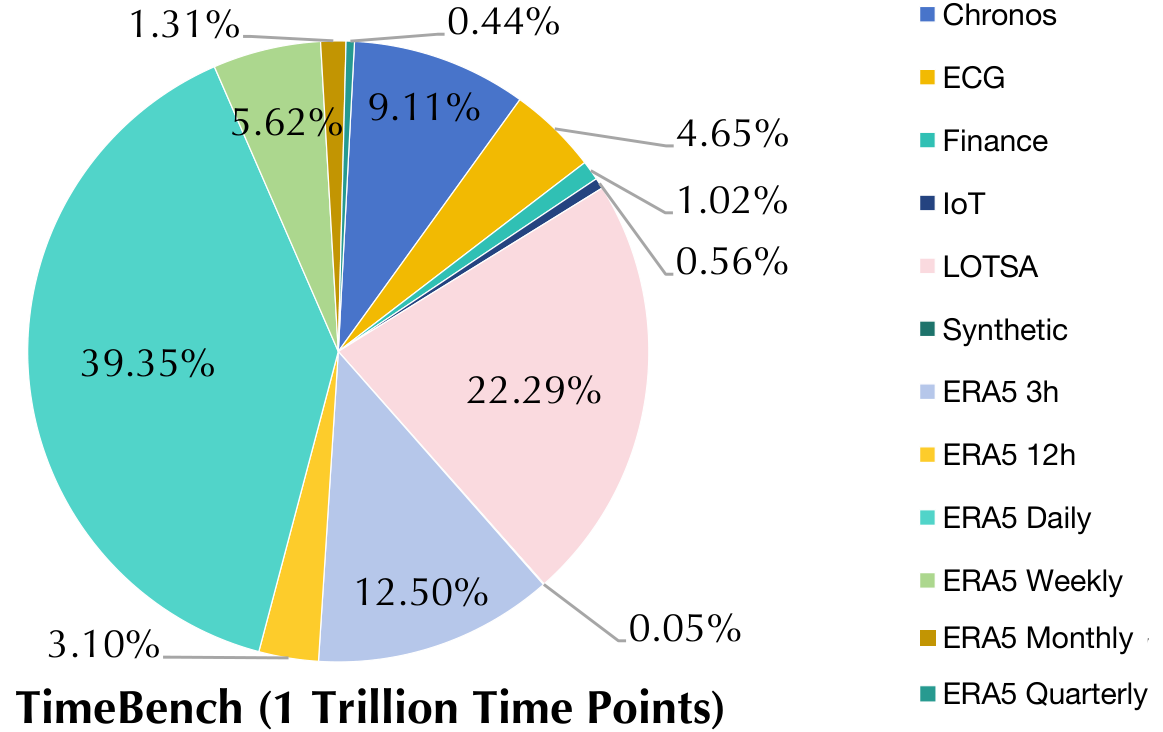
We collected and curated TimeBench, which comprises over a trillion time points from various sources, as shown in Figure 3. Several datasets originate from research teams (Woo et al., 2024; Ansari et al., 2024; Liu et al., 2024b; Liu et al., 2024c). While most datasets are collected from real-world records, a small portion (0.05%) is generated synthetically to enhance pattern diversity, following KernelSynth proposed by Ansari et al. (2024). We also leverage substantial meteorological data (Hersbach et al., 2020) because of the predictability of weather systems. Data of different frequencies encompasses common and comprehensive temporal dynamics.
We evaluate Sundial on best-recognized zero-shot forecasting benchmarks (Section 5.1) and investigate the scaling behavior of Sundial (Section 5.2). We compare TimeFlow with other training objectives (Section 5.3). We delve into test-time calibration of generative forecasters (Section 5.4). We conduct model adaptation of Sundial, i.e., instruction tuning (Section 5.5) and provide in-depth ablation studies to evaluate our modular enhancement (Section 5.6).
| Models | Timer-XL | TimesFM | ||||||||||||||||||||||
| (Ours) | (Ours) | (Ours) | (2024b) | (2024b) | (2024b) | (2024b) | (2024) | (2024) | (2024) | (2024) | (2023b) | |||||||||||||
| Metric | MSE | MAE | MSE | MAE | MSE | MAE | MSE | MAE | MSE | MAE | MSE | MAE | MSE | MAE | MSE | MAE | MSE | MAE | MSE | MAE | MSE | MAE | MSE | MAE |
| ETTm1 | 0.354 | 0.388 | 0.336 | 0.377 | 0.331 | 0.369 | 0.394 | 0.415 | 0.376 | 0.405 | 0.356 | 0.391 | 0.373 | 0.392 | 0.406 | 0.385 | 0.422 | 0.391 | 0.645 | 0.500 | 0.555 | 0.465 | 0.433 | 0.418 |
| ETTm2 | 0.265 | 0.324 | 0.258 | 0.320 | 0.254 | 0.315 | 0.317 | 0.365 | 0.316 | 0.361 | 0.288 | 0.344 | 0.273 | 0.336 | 0.311 | 0.337 | 0.329 | 0.343 | 0.310 | 0.350 | 0.295 | 0.338 | 0.328 | 0.346 |
| ETTh1 | 0.390 | 0.418 | 0.411 | 0.434 | 0.395 | 0.420 | 0.400 | 0.424 | 0.394 | 0.419 | 0.412 | 0.426 | 0.404 | 0.417 | 0.417 | 0.419 | 0.480 | 0.439 | 0.591 | 0.468 | 0.588 | 0.466 | 0.473 | 0.443 |
| ETTh2 | 0.340 | 0.387 | 0.333 | 0.387 | 0.334 | 0.387 | 0.366 | 0.404 | 0.405 | 0.415 | 0.371 | 0.399 | 0.347 | 0.388 | 0.362 | 0.382 | 0.367 | 0.377 | 0.405 | 0.410 | 0.455 | 0.427 | 0.392 | 0.406 |
| ECL | 0.169 | 0.265 | 0.169 | 0.265 | 0.166 | 0.262 | - | - | - | - | - | - | 0.174 | 0.278 | 0.187 | 0.274 | 0.186 | 0.270 | 0.214 | 0.278 | 0.204 | 0.273 | - | - |
| Weather | 0.233 | 0.271 | 0.234 | 0.270 | 0.238 | 0.275 | 0.265 | 0.297 | 0.270 | 0.300 | 0.256 | 0.288 | 0.256 | 0.294 | 0.287 | 0.281 | 0.264 | 0.273 | 0.292 | 0.315 | 0.279 | 0.306 | - | - |
| Count | 7 | 2 | 8 | 5 | 16 | 16 | 0 | 1 | 0 | 0 | 2 | 1 | 1 | 3 | 0 | 2 | 0 | 6 | 0 | 0 | 0 | 0 | 0 | 0 |
View original table
| Type | Statistical Methods | Task-Specific Models (Superwised) | Time Series Foundation Models (Zero-Shot) | |||||||||||
|---|---|---|---|---|---|---|---|---|---|---|---|---|---|---|
| Model | Naïve | Seasonal | Auto | Auto | DeepAR | TiDE | N-BEATS | PTST. | iTrans. | TimesFM | TabPFN | Chronos | Moirai | Sundial |
| Naïve | ARIMA | Theta | (2020) | (2023a) | (2019) | (2022) | (2023a) | (2023b) | (2025) | (2024) | (2024) | (Ours) | ||
| MASE | 1.260 | 1.000 | 0.964 | 0.978 | 1.206 | 0.980 | 0.842 | 0.762 | 0.802 | 0.680 | 0.748 | 0.786 | 0.809 | 0.673 |
| CRPS | 1.383 | 1.000 | 0.770 | 1.051 | 0.721 | 0.652 | 0.689 | 0.496 | 0.524 | 0.465 | 0.480 | 0.551 | 0.515 | 0.472 |
| Rank | 28.072 | 26.175 | 21.515 | 24.031 | 18.938 | 18.557 | 21.381 | 10.052 | 11.320 | 8.237 | 8.268 | 14.309 | 10.175 | 9.062 |
View original table

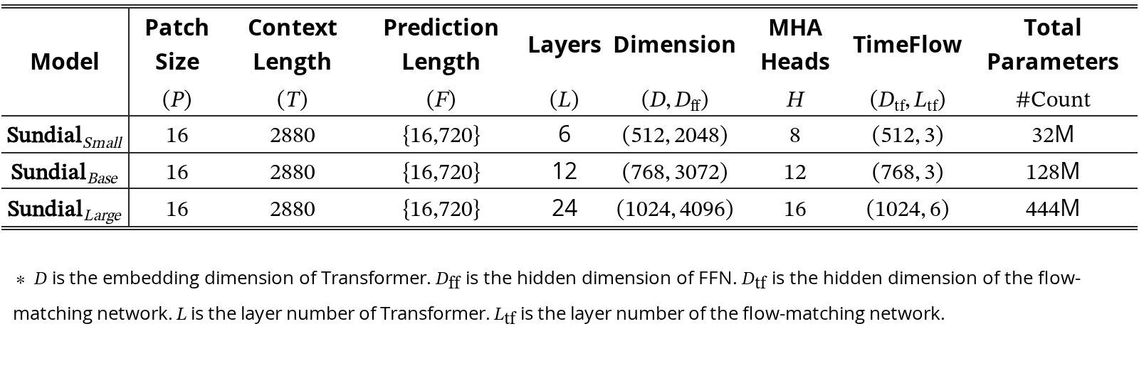
In this section, we focus on zero-shot forecasting, we compare Sundial with advanced time series foundation models on various benchmarks, including (1) point forecasting: we adopt the long-term forecasting benchmark (Wu et al., 2022), which assesses the performance under different forecasting horizons using MSE and MAE; (2) probabilistic forecasting: we experiment on GIFT-Eval (Aksu et al., 2024) and FEV leaderboard (Ansari et al., 2024), following their official evaluation suite and assessing point (MASE) and probabilistic (CRPS and WQL) metrics. All evaluated datasets are excluded from the pre-training dataset. Model is available on HuggingFace and configurations are detailed in Table 5.
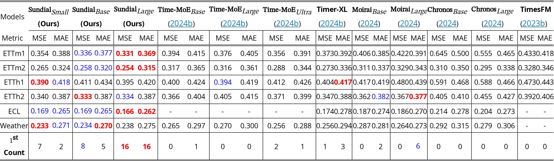
As shown in Table 1, Sundial consistently outperforms other advanced time series foundation models. Compared with the previous state-of-the-art model Time-MoE (Shi et al., 2024b), the Sundial family using fewer parameters achieves the average MSE reduction of and averaged MAE reduction of . Notably, continuous tokenization allows our model to conduct patch-level forecasting with fewer autoregression steps, while Chronos using point-wise discrete tokenization may not be suitable in long-term forecasting.
Beyond point forecasting, Sundial possesses a unique generative capability for making probabilistic predictions. Following Ansari et al. (2024), we calculate the median and quantiles using a set of raw predictions of Sundial. While several baseline models have been pre-trained by the consistent objective function for probabilistic evaluation, e.g., quantile loss for WQL, Sundial calculates these statistics for evaluation without any prior knowledge.
Aggregated results are presented in Table 2. The benchmark evaluates performance from datasets and baseline models, encompassing statistical methods, task-specific models, and time series foundation models. Among supervised models and advanced foundation models, Sundial attains the first place in MASE and second place in CRPS on all unseen datasets. While the top PatchTST (Nie et al., 2022) is exhaustively trained and tweaked on each dataset, the zero-shot performance of Sundial highlights its simplicity and robustness on this comprehensive benchmark.
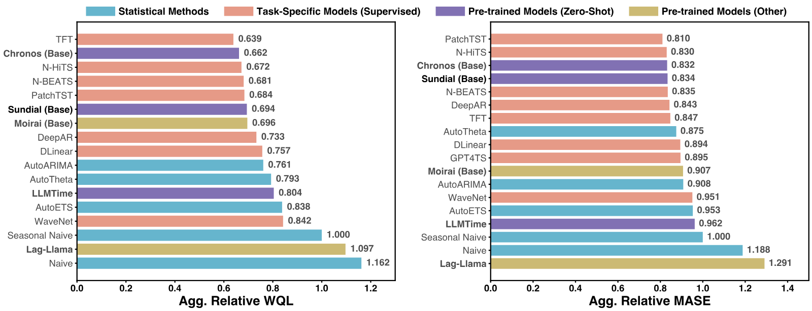
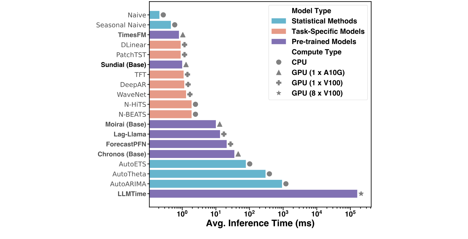
We evaluate our Sundial on the open leaderboard established by AutoGluon (Ansari et al., 2024), which includes datasets for probabilistic forecasting. As shown in Figure 4, the zero-shot forecasting performance of Sundial exceeds statistical methods and deep models that are superwisedly trained in distribution. While Sundial is ranked as the second zero-shot pre-trained models after Chronos, Sundial realizes inference speedup as shown in Figure 5. Based on patch-wise tokenization and multi-patch prediction, our inference speed is near to N-BEATS.
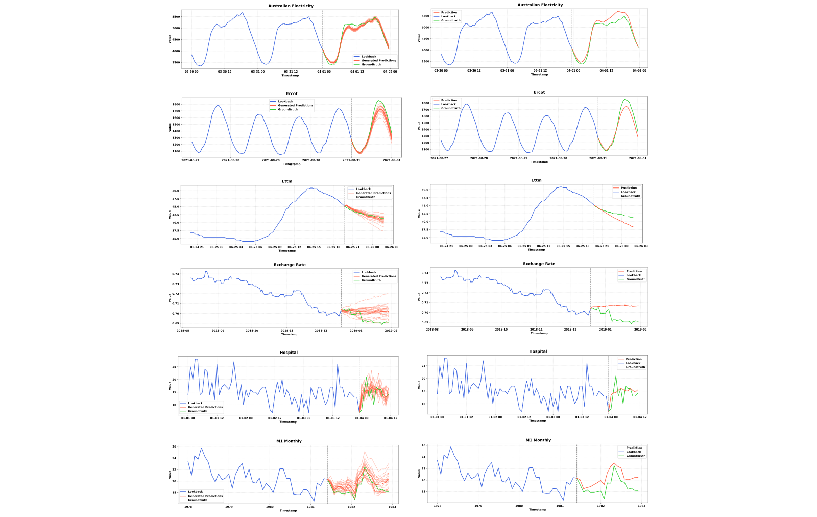
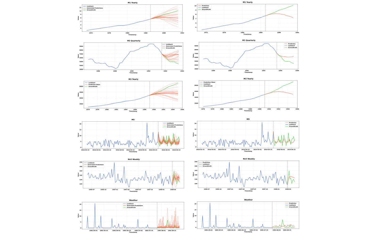
Besides, we provide qualitative showcases in Appendix D. TimeFlow can generate highly eventful and coherent temporal patterns with input series. Beyond the mean or quantiles, our model enables the estimation of arbitrary statistics by sampling directly from the predictive distribution.
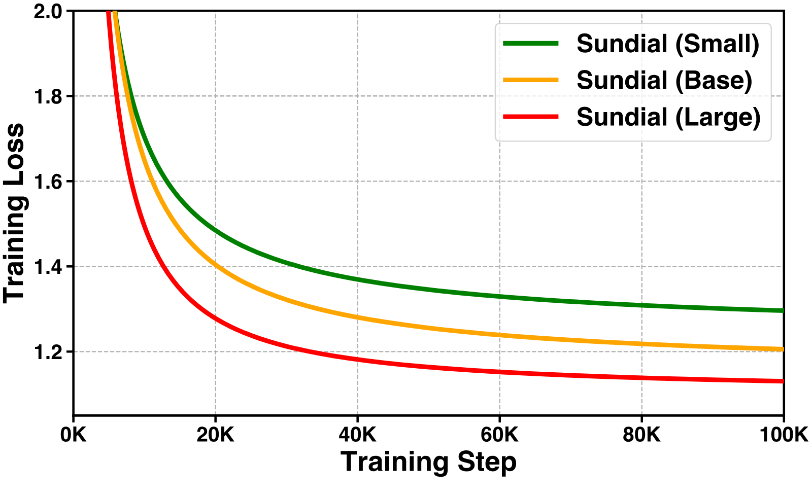
From Table 1, the larger Sundial model consistently achieves better performance with the scaling of parameters. Beyond downstream performance, we delve into the utilization of model capacity. Figure 6 shows training curves of different sizes. Compared to Sundial (Small), the large version leads to reduction in the converged training loss, exhibiting promising model capacity of generative forecasters.
Based on the flow-matching framework, TimeFlow Loss allows autoregressive models to learn and generate flexible distributions while enhancing representation learning. To validate the effectiveness of this design, we implement two alternatives: (1) an MLP network and MSE Loss and (2) a parameterized training objective based on the denoising diffusion procedure (Li et al., 2024). We adopt the same parameterized network and Transformer backbone and pre-train them on TimeBench. Since the converged training loss is not comparable across different objective functions, we compare zero-shot performance in Table 3. Despite allowing for sampling predictions, performance using diffusion-based objective is notably inferior to TimeFlow Loss.
| Objective | ETTm1 | ETTm2 | ETTh1 | ETTh2 | ECL | Weather | Avg. |
|---|---|---|---|---|---|---|---|
| TimeFlow | 0.336 | 0.258 | 0.411 | 0.333 | 0.169 | 0.234 | 0.290 |
| Diffusion | 0.362 | 0.265 | 0.444 | 0.360 | 0.202 | 0.252 | 0.314 |
| MSE | 0.360 | 0.264 | 0.404 | 0.341 | 0.175 | 0.231 | 0.296 |
View original table

In addition to zero-shot performance, we provide showcases for quality evaluations in Appendix D.2. Pre-trained models optimized by the specific MSE Loss can only output a single prediction. And the prediction is sometimes over-smooth due to mode collapse (refer to Appendix C.1). Instead, generative modeling can accommodate significantly different future variations even if their lookback series are similar. We also provide a probablistic metric CRPS to compare different objectives in Table 7, which validate that the predictive distribution modeled by TimeFlow is more coherent and diverse than counterpart training objectives. It benefits downstream tasks by generating multiple plausible predictions, conveys various future possibilities and enhances the reliability of decision-making.
Generative modeling facilitates the flexibility to calibrate the final prediction during inference. Based on the median-based forecasting strategy, i.e., starting from multiple noise of a standard Gaussian and calculating the median of raw predictions, there are two configurations to calibrate final predictions: (1) the number of samples to calculate statistics and (2) sampling steps used for flow-matching. Figure 7 shows the results using different configurations.
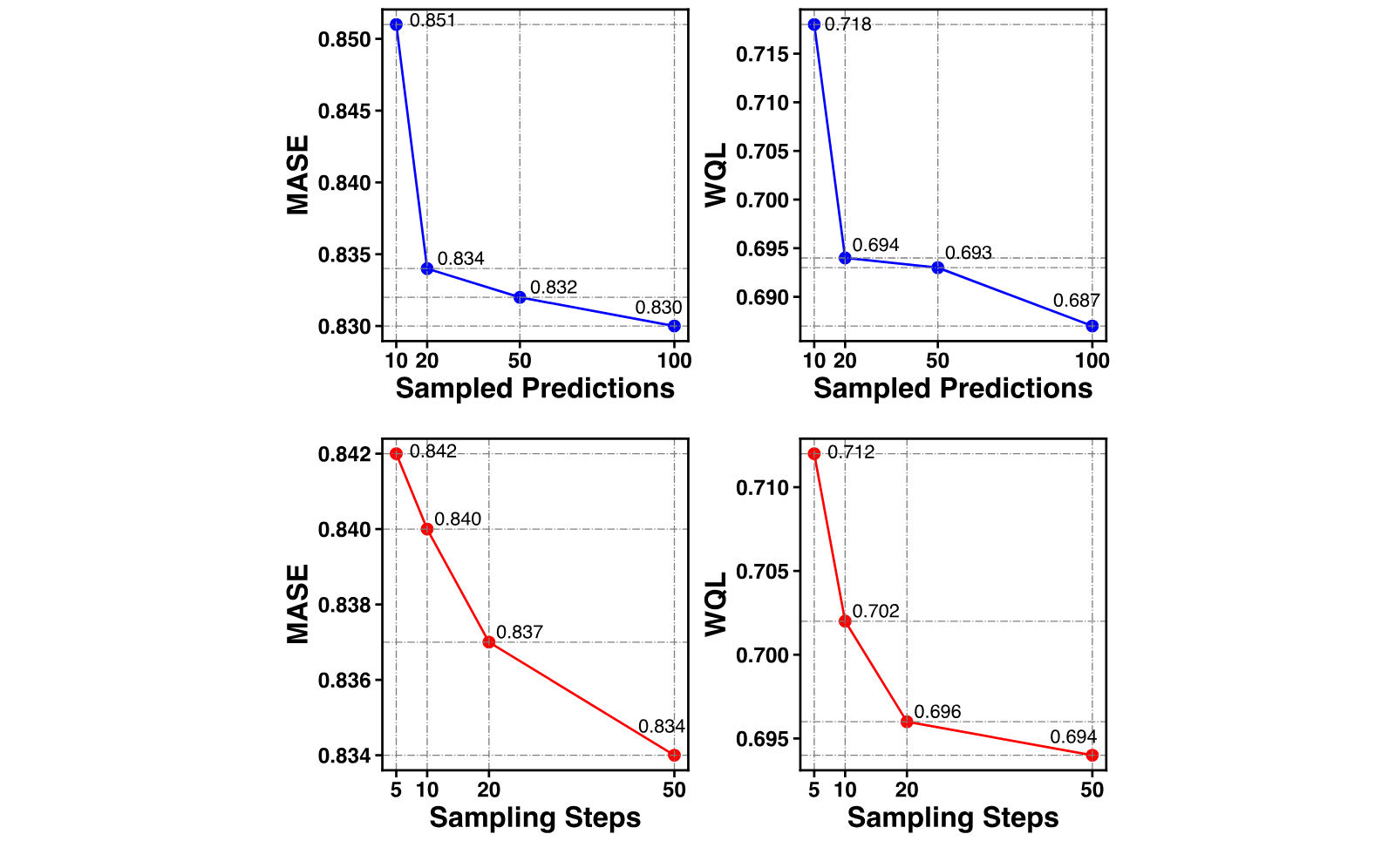
The top two figures conform to the central limit theorem. Generating more samples leads to more calibrated estimation of prediction and confidence interval. The bottom two figures indicate that using fine-grained steps during the push-forward process can leads to more precise predictions.
The trade-off between inference time and performance reveals the potential of test-time calibration, which does not require retraining models. The generative capability of Sundial provides flexibility for various use cases requiring different levels of uncertainty. In our experiments, sampling predictions with each generated by steps consumes nearly one second on a CPU, which is notably more efficient than tuning deep models or statistical methods. Advanced strategies of sampling and post-processing of raw prediction leave interesting directions for future exploration.
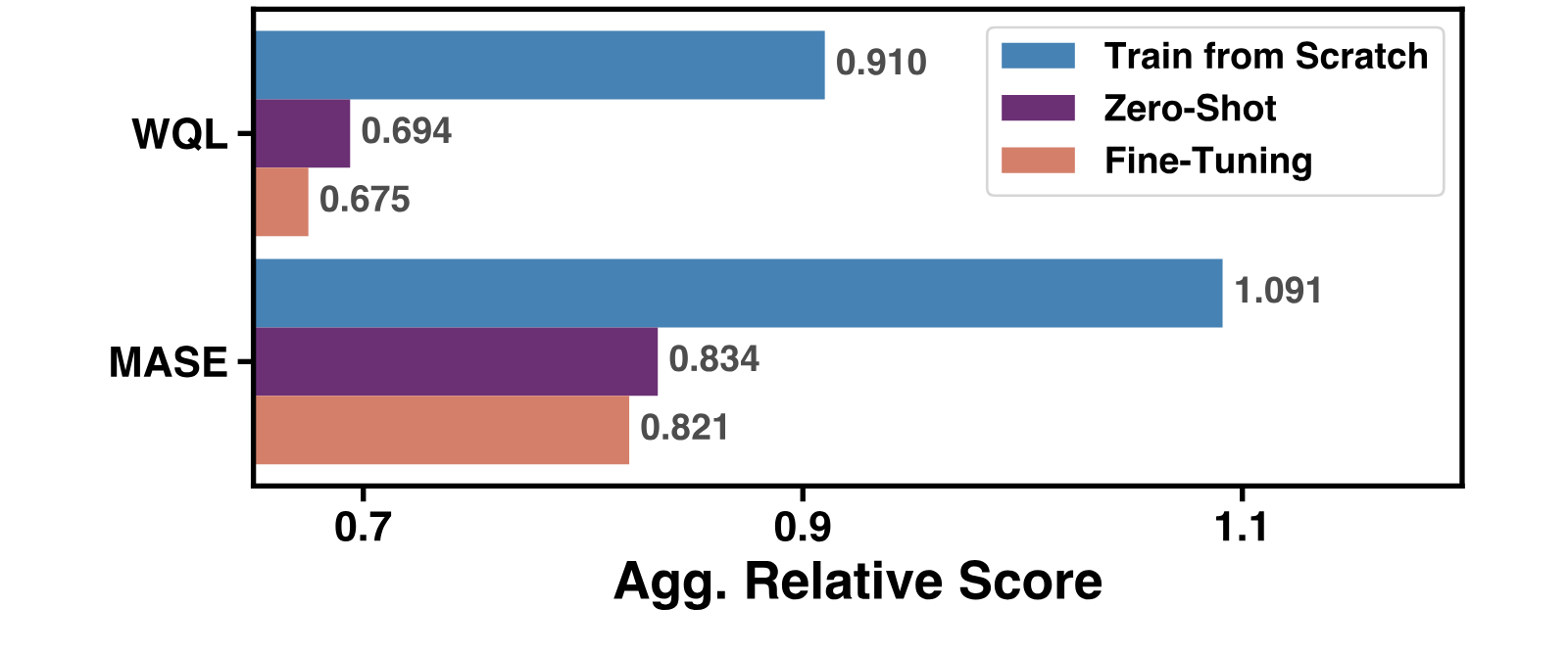
Inspired by the prevalence of instruction tuning (Wei et al., 2021) that adapts foundation models on a collection of tasks. We fine-tune pre-trained Sundial (Base) on the FEV leaderboard, including short-term tasks with different prediction lengths. Our model is tuned once on all aggregated datasets. We evaluate the performance on unseen test splits (Figure 8). We observe that the performance can be further improved compared to zero-shot forecasting. Furthermore, training from scratch on aggregated datasets results in inferior performance, implying knowledge transfer in pre-trained models.
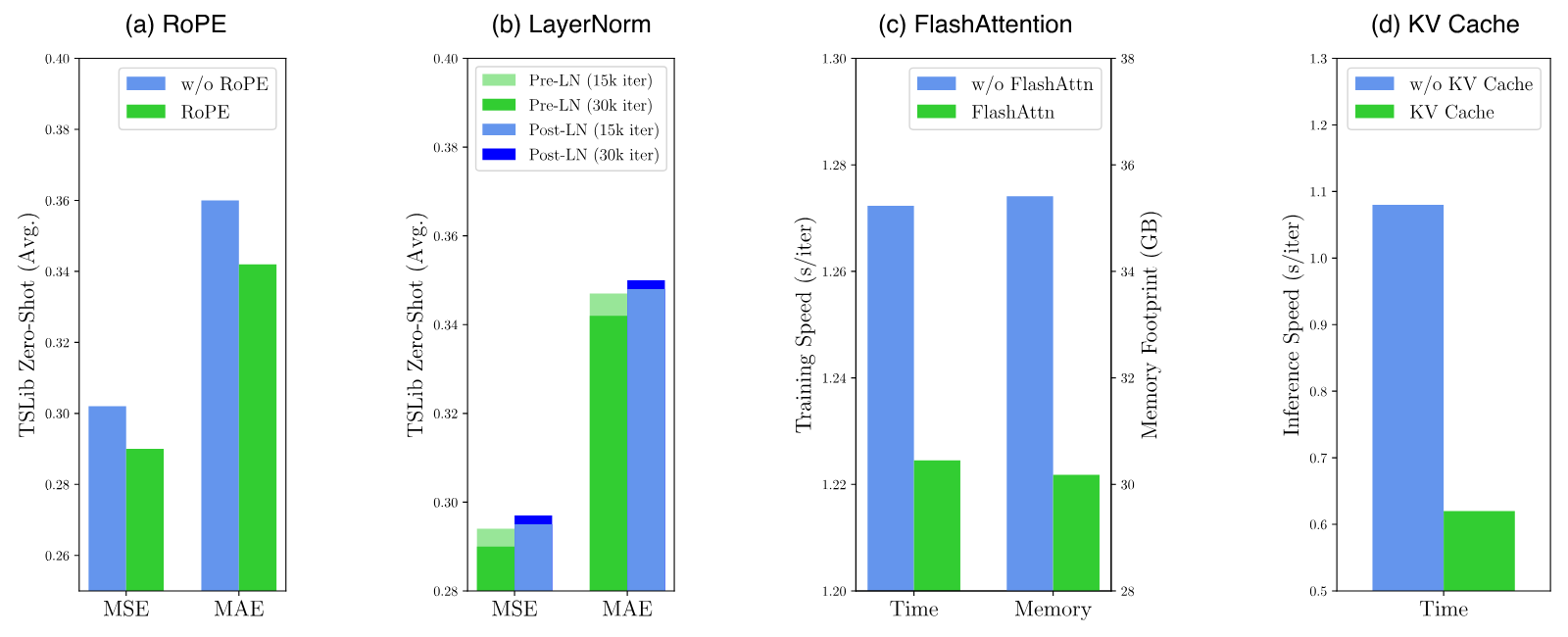
We conducted several ablation studies that provide insights into the enhancement made to Sundial’s architecture. We evaluate the overall zero-shot performance on TSLib, which covers six different datasets and four prediction lengths.
Prior research (Liu et al., 2024b) observed that the introduction of RoPE (Su et al., 2024) yields better results in supervised forecasting tasks. As shown in Figure 9 (a), RoPE can also improve zero-shot forecasting, presenting a general enhancement for time series foundation models.
Pre-LN (Baevski and Auli, 2018) is widely adopted in large language models (Touvron et al., 2023) due to the training stability. As depicted in Figure 9 (b), training with Pre-LN for more iterations yield better performance. In contrast, training with Post-LN, which is the predominant choice in supervised models, may adversely affect downstream results.
We make it to leverage FlashAttention (Dao et al., 2022) and KV Cache to reduce the computational costs. As shown in Figure 9 (c) and (d), they notably reduce memory footprint and inference time without affecting performance.
In this work, we collect and curate TimeBench, a trillion-scale time series dataset for building time series foundation models, which can benefit the research community. Towards time series foundation models, we delve into tokenization and optimization, presenting contributions in two aspects. First, we demonstrate that continuous tokenization, such as patch tokens, can be more effective and efficient for the time series modality, and generative modeling presents a native approach for learning on continuous-valued time series. Second, we propose a novel training objective to accommodate heterogeneous time series distribution. It endows autoregressive models with an inherent capability to sample from non-categorical distribution. Our pre-trained Sundial models make substantial advances on best-recognized forecasting leaderboards. We hope this work can inspire future paradigms for pre-training time series foundation models and enhance their applicability to real-world applications.
This work was supported by the National Natural Science Foundation of China (U2342217 and 62021002), State Grid Ningxia Electric Power Co. Science and Technology Project (SGNXYX00SCJS2400058), and the BNRist Innovation Fund (BNR2024RC01010), the National Engineering Research Center for Big Data Software.
We extend our gratitude to Xingzhuo Guo for his expertise in flow-matching and meticulous proofreading of the method section. We further thank Jialong Wu, Yuezhou Ma and Yu Zhang for insightful discussions about generative models. Their collective support significantly enhanced this work.
This paper aims to advance the development of time series foundation models. We curated a pre-training dataset from publicly available resources. Our models employ an efficient tokenization and incorporate a generative training objective. The proposed TimeFlow Loss provides insights for training generative foundation models for time series forecasting. We released our pre-trained models that demonstrate notable zero-shot forecasting performance. The generative forecasting paradigm enhances the model reliability for decision-making. Our paper mainly focuses on scientific research and has no obvious negative social impact.
References
- Aksu et al. (2024) T. Aksu, G. Woo, J. Liu, X. Liu, C. Liu, S. Savarese, C. Xiong, and D. Sahoo GIFT-eval: a benchmark for general time series forecasting model evaluation. In NeurIPS Workshop on Time Series in the Age of Large Models, Cited by: Appendix B, §C.1, §1, §1, §5.1, Table 2.
- Ansari et al. (2024) A. F. Ansari, L. Stella, C. Turkmen, X. Zhang, P. Mercado, H. Shen, O. Shchur, S. S. Rangapuram, S. P. Arango, S. Kapoor, et al. Chronos: learning the language of time series. arXiv preprint arXiv:2403.07815. Cited by: Table 4, Table 4, Appendix A, Table 6, Appendix B, §C.2, §C.4, §C.5, Figure 11, Figure 12, §D.1, Table 9, Table 9, §1, §1, §1, §2.1, §2.2, §4.1.1, §4.2, Figure 4, Figure 5, §5.1.2, §5.1.2, §5.1, Table 1, Table 1, Table 2.
- Baevski and Auli (2018) A. Baevski and M. Auli Adaptive input representations for neural language modeling. arXiv preprint arXiv:1809.10853. Cited by: §5.6.
- Bai et al. (2018) S. Bai, J. Z. Kolter, and V. Koltun An empirical evaluation of generic convolutional and recurrent networks for sequence modeling. arXiv preprint arXiv:1803.01271. Cited by: §2.1.
- Bengio et al. (2000) Y. Bengio, R. Ducharme, and P. Vincent A neural probabilistic language model. Advances in neural information processing systems 13. Cited by: §1.
- Bommasani et al. (2021) R. Bommasani, D. A. Hudson, E. Adeli, R. Altman, S. Arora, S. von Arx, M. S. Bernstein, J. Bohg, A. Bosselut, E. Brunskill, et al. On the opportunities and risks of foundation models. arXiv preprint arXiv:2108.07258. Cited by: §1, §2.1.
- Box et al. (2015) G. E. Box, G. M. Jenkins, G. C. Reinsel, and G. M. Ljung Time series analysis: forecasting and control. John Wiley & Sons. Cited by: §1.
- Box (2013) G. Box Box and jenkins: time series analysis, forecasting and control. In A Very British Affair: Six Britons and the Development of Time Series Analysis During the 20th Century, pp. 161–215. Cited by: §1.
- Dao et al. (2022) T. Dao, D. Fu, S. Ermon, A. Rudra, and C. Ré Flashattention: fast and memory-efficient exact attention with io-awareness. Advances in Neural Information Processing Systems 35, pp. 16344–16359. Cited by: §1, §4.1.2, §5.6.
- Das et al. (2023a) A. Das, W. Kong, A. Leach, R. Sen, and R. Yu Long-term forecasting with tide: time-series dense encoder. arXiv preprint arXiv:2304.08424. Cited by: Table 2.
- Das et al. (2023b) A. Das, W. Kong, R. Sen, and Y. Zhou A decoder-only foundation model for time-series forecasting. arXiv preprint arXiv:2310.10688. Cited by: Appendix A, Table 6, §C.4, Table 9, §1, §2.2, §4.1.3, Table 1, Table 2.
- Esser et al. (2024) P. Esser, S. Kulal, A. Blattmann, R. Entezari, J. Müller, H. Saini, Y. Levi, D. Lorenz, A. Sauer, F. Boesel, et al. Scaling rectified flow transformers for high-resolution image synthesis. In Forty-first International Conference on Machine Learning, Cited by: §2.3, §3.2.
- Goldberger et al. (2000) A. L. Goldberger, L. A. Amaral, L. Glass, J. M. Hausdorff, P. C. Ivanov, R. G. Mark, J. E. Mietus, G. B. Moody, C. Peng, and H. E. Stanley PhysioBank, physiotoolkit, and physionet: components of a new research resource for complex physiologic signals. circulation 101 (23), pp. e215–e220. Cited by: Table 4, Appendix A.
- Goswami et al. (2024) M. Goswami, K. Szafer, A. Choudhry, Y. Cai, S. Li, and A. Dubrawski MOMENT: a family of open time-series foundation models. arXiv preprint arXiv:2402.03885. Cited by: Table 6.
- Gruver et al. (2024) N. Gruver, M. Finzi, S. Qiu, and A. G. Wilson Large language models are zero-shot time series forecasters. Advances in Neural Information Processing Systems 36. Cited by: Table 6.
- Gruver et al. (2023) N. Gruver, M. Finzi, S. Qiu, and A. G. Wilson Large language models are zero-shot time series forecasters. arXiv preprint arXiv:2310.07820. Cited by: §1.
- Hersbach et al. (2020) H. Hersbach, B. Bell, P. Berrisford, S. Hirahara, A. Horányi, J. Muñoz-Sabater, J. Nicolas, C. Peubey, R. Radu, D. Schepers, et al. The era5 global reanalysis. Quarterly Journal of the Royal Meteorological Society 146 (730), pp. 1999–2049. Cited by: §4.2.
- Hoo et al. (2025) S. B. Hoo, S. Müller, D. Salinas, and F. Hutter The tabular foundation model tabpfn outperforms specialized time series forecasting models based on simple features. arXiv preprint arXiv:2501.02945. Cited by: Table 2.
- Hyndman (2018) R. Hyndman Forecasting: principles and practice. OTexts. Cited by: §1, §2.1.
- Ke et al. (2017) G. Ke, Q. Meng, T. Finley, T. Wang, W. Chen, W. Ma, Q. Ye, and T. Liu Lightgbm: a highly efficient gradient boosting decision tree. Advances in neural information processing systems 30. Cited by: §2.1.
- Kim et al. (2021) T. Kim, J. Kim, Y. Tae, C. Park, J. Choi, and J. Choo Reversible instance normalization for accurate time-series forecasting against distribution shift. In International Conference on Learning Representations, Cited by: §2.1.
- Kingma and Ba (2014) D. P. Kingma and J. Ba Adam: a method for stochastic optimization. arXiv preprint arXiv:1412.6980. Cited by: Appendix B.
- Kollovieh et al. (2024) M. Kollovieh, M. Lienen, D. Lüdke, L. Schwinn, and S. Günnemann Flow matching with gaussian process priors for probabilistic time series forecasting. arXiv preprint arXiv:2410.03024. Cited by: §2.3.
- Li et al. (2024) T. Li, Y. Tian, H. Li, M. Deng, and K. He Autoregressive image generation without vector quantization. arXiv preprint arXiv:2406.11838. Cited by: §1, §5.3.
- Liang et al. (2024) Y. Liang, H. Wen, Y. Nie, Y. Jiang, M. Jin, D. Song, S. Pan, and Q. Wen Foundation models for time series analysis: a tutorial and survey. In Proceedings of the 30th ACM SIGKDD conference on knowledge discovery and data mining, pp. 6555–6565. Cited by: §2.2.
- Lim et al. (2021) B. Lim, S. Ö. Arık, N. Loeff, and T. Pfister Temporal fusion transformers for interpretable multi-horizon time series forecasting. International Journal of Forecasting 37 (4), pp. 1748–1764. Cited by: §2.1.
- Lipman et al. (2022) Y. Lipman, R. T. Chen, H. Ben-Hamu, M. Nickel, and M. Le Flow matching for generative modeling. arXiv preprint arXiv:2210.02747. Cited by: §1, §2.3, §3.1.
- Lipman et al. (2024) Y. Lipman, M. Havasi, P. Holderrieth, N. Shaul, M. Le, B. Karrer, R. T. Chen, D. Lopez-Paz, H. Ben-Hamu, and I. Gat Flow matching guide and code. arXiv preprint arXiv:2412.06264. Cited by: §2.3.
- Liu et al. (2024a) Y. Liu, K. Zhang, Y. Li, Z. Yan, C. Gao, R. Chen, Z. Yuan, Y. Huang, H. Sun, J. Gao, et al. Sora: a review on background, technology, limitations, and opportunities of large vision models. arXiv preprint arXiv:2402.17177. Cited by: §1, §2.3.
- Liu et al. (2023a) Y. Liu, T. Hu, H. Zhang, H. Wu, S. Wang, L. Ma, and M. Long Itransformer: inverted transformers are effective for time series forecasting. arXiv preprint arXiv:2310.06625. Cited by: §1, Table 2.
- Liu et al. (2023b) Y. Liu, C. Li, J. Wang, and M. Long Koopa: learning non-stationary time series dynamics with koopman predictors. arXiv preprint arXiv:2305.18803. Cited by: §2.1.
- Liu et al. (2024b) Y. Liu, G. Qin, X. Huang, J. Wang, and M. Long Timer-xl: long-context transformers for unified time series forecasting. arXiv preprint arXiv:2410.04803. Cited by: Appendix A, Table 6, §C.4, Table 9, §2.2, §4.2, §5.6, Table 1.
- Liu et al. (2022) Y. Liu, H. Wu, J. Wang, and M. Long Non-stationary transformers: exploring the stationarity in time series forecasting. Advances in Neural Information Processing Systems 35, pp. 9881–9893. Cited by: §4.1.1.
- Liu et al. (2024c) Y. Liu, H. Zhang, C. Li, X. Huang, J. Wang, and M. Long Timer: generative pre-trained transformers are large time series models. In Forty-first International Conference on Machine Learning, Cited by: Appendix A, Appendix A, Appendix B, §C.4, §1, §2.2, §4.2, §4.
- Muñoz-Sabater et al. (2021) J. Muñoz-Sabater, E. Dutra, A. Agustí-Panareda, C. Albergel, G. Arduini, G. Balsamo, S. Boussetta, M. Choulga, S. Harrigan, H. Hersbach, et al. ERA5-land: a state-of-the-art global reanalysis dataset for land applications. Earth system science data 13 (9), pp. 4349–4383. Cited by: Table 4, Table 4, Table 4, Table 4, Table 4, Table 4, Appendix A.
- Nie et al. (2022) Y. Nie, N. H. Nguyen, P. Sinthong, and J. Kalagnanam A time series is worth 64 words: long-term forecasting with transformers. arXiv preprint arXiv:2211.14730. Cited by: §1, §2.1, §5.1.2, Table 2.
- OpenAI (2023) R. OpenAI Gpt-4 technical report. arxiv 2303.08774. View in Article 2, pp. 13. Cited by: §1, §3.2.
- Oreshkin et al. (2019) B. N. Oreshkin, D. Carpov, N. Chapados, and Y. Bengio N-beats: neural basis expansion analysis for interpretable time series forecasting. arXiv preprint arXiv:1905.10437. Cited by: §1, Table 2.
- Paszke et al. (2019) A. Paszke, S. Gross, F. Massa, A. Lerer, J. Bradbury, G. Chanan, T. Killeen, Z. Lin, N. Gimelshein, L. Antiga, et al. Pytorch: an imperative style, high-performance deep learning library. Advances in neural information processing systems 32. Cited by: Appendix B.
- Peebles and Xie (2023) W. Peebles and S. Xie Scalable diffusion models with transformers. In Proceedings of the IEEE/CVF International Conference on Computer Vision, pp. 4195–4205. Cited by: §4.1.3.
- [41] PEMS Traffic Dataset. Note: http://pems.dot.ca.gov/ Cited by: Table 9.Source
- Pope et al. (2023) R. Pope, S. Douglas, A. Chowdhery, J. Devlin, J. Bradbury, J. Heek, K. Xiao, S. Agrawal, and J. Dean Efficiently scaling transformer inference. Proceedings of Machine Learning and Systems 5, pp. 606–624. Cited by: §1, §4.1.2.
- Radford et al. (2018) A. Radford, K. Narasimhan, T. Salimans, I. Sutskever, et al. Improving language understanding by generative pre-training. OpenAI. Cited by: §1.
- Ramesh et al. (2021) A. Ramesh, M. Pavlov, G. Goh, S. Gray, C. Voss, A. Radford, M. Chen, and I. Sutskever Zero-shot text-to-image generation. In International conference on machine learning, pp. 8821–8831. Cited by: §1.
- Rasley et al. (2020) J. Rasley, S. Rajbhandari, O. Ruwase, and Y. He Deepspeed: system optimizations enable training deep learning models with over 100 billion parameters. In Proceedings of the 26th ACM SIGKDD International Conference on Knowledge Discovery & Data Mining, pp. 3505–3506. Cited by: §4.1.2.
- Rasul et al. (2023) K. Rasul, A. Ashok, A. R. Williams, A. Khorasani, G. Adamopoulos, R. Bhagwatkar, M. Biloš, H. Ghonia, N. V. Hassen, A. Schneider, et al. Lag-llama: towards foundation models for time series forecasting. arXiv preprint arXiv:2310.08278. Cited by: Table 6.
- Rasul et al. (2021) K. Rasul, C. Seward, I. Schuster, and R. Vollgraf Autoregressive denoising diffusion models for multivariate probabilistic time series forecasting. In International Conference on Machine Learning, pp. 8857–8868. Cited by: §2.3.
- Rombach et al. (2022) R. Rombach, A. Blattmann, D. Lorenz, P. Esser, and B. Ommer High-resolution image synthesis with latent diffusion models. In Proceedings of the IEEE/CVF conference on computer vision and pattern recognition, pp. 10684–10695. Cited by: §3.2.
- Salinas et al. (2020) D. Salinas, V. Flunkert, J. Gasthaus, and T. Januschowski DeepAR: probabilistic forecasting with autoregressive recurrent networks. International journal of forecasting 36 (3), pp. 1181–1191. Cited by: §2.1, Table 2.
- Shen and Kwok (2023) L. Shen and J. Kwok Non-autoregressive conditional diffusion models for time series prediction. In International Conference on Machine Learning, pp. 31016–31029. Cited by: §2.3.
- Shi et al. (2024a) J. Shi, Q. Ma, H. Ma, and L. Li Scaling law for time series forecasting. arXiv preprint arXiv:2405.15124. Cited by: Appendix A.
- Shi et al. (2024b) X. Shi, S. Wang, Y. Nie, D. Li, Z. Ye, Q. Wen, and M. Jin Time-moe: billion-scale time series foundation models with mixture of experts. arXiv preprint arXiv:2409.16040. Cited by: Appendix A, Table 6, §C.4, Table 9, Table 9, Table 9, Table 9, §2.2, §5.1.1, Table 1, Table 1, Table 1, Table 1.
- Shoeybi et al. (2019) M. Shoeybi, M. Patwary, R. Puri, P. LeGresley, J. Casper, and B. Catanzaro Megatron-lm: training multi-billion parameter language models using model parallelism. arXiv preprint arXiv:1909.08053. Cited by: §4.1.2.
- Sohl-Dickstein et al. (2015) J. Sohl-Dickstein, E. Weiss, N. Maheswaranathan, and S. Ganguli Deep unsupervised learning using nonequilibrium thermodynamics. In International conference on machine learning, pp. 2256–2265. Cited by: §2.3.
- Su et al. (2024) J. Su, M. Ahmed, Y. Lu, S. Pan, W. Bo, and Y. Liu Roformer: enhanced transformer with rotary position embedding. Neurocomputing 568, pp. 127063. Cited by: §1, §4.1.2, §5.6.
- Tashiro et al. (2021) Y. Tashiro, J. Song, Y. Song, and S. Ermon Csdi: conditional score-based diffusion models for probabilistic time series imputation. Advances in Neural Information Processing Systems 34, pp. 24804–24816. Cited by: §2.3.
- Tong et al. (2023) A. Tong, K. Fatras, N. Malkin, G. Huguet, Y. Zhang, J. Rector-Brooks, G. Wolf, and Y. Bengio Improving and generalizing flow-based generative models with minibatch optimal transport. arXiv preprint arXiv:2302.00482. Cited by: §1.
- Touvron et al. (2023) H. Touvron, T. Lavril, G. Izacard, X. Martinet, M. Lachaux, T. Lacroix, B. Rozière, N. Goyal, E. Hambro, F. Azhar, et al. Llama: open and efficient foundation language models. arXiv preprint arXiv:2302.13971. Cited by: §5.6.
- Vovk et al. (2005) V. Vovk, A. Gammerman, and G. Shafer Algorithmic learning in a random world. Vol. 29, Springer. Cited by: §3.2.
- Wei et al. (2021) J. Wei, M. Bosma, V. Y. Zhao, K. Guu, A. W. Yu, B. Lester, N. Du, A. M. Dai, and Q. V. Le Finetuned language models are zero-shot learners. arXiv preprint arXiv:2109.01652. Cited by: §5.5.
- Wen et al. (2017) R. Wen, K. Torkkola, B. Narayanaswamy, and D. Madeka A multi-horizon quantile recurrent forecaster. arXiv preprint arXiv:1711.11053. Cited by: §1, §2.2.
- Woo et al. (2024) G. Woo, C. Liu, A. Kumar, C. Xiong, S. Savarese, and D. Sahoo Unified training of universal time series forecasting transformers. arXiv preprint arXiv:2402.02592. Cited by: Table 4, Appendix A, Table 6, Appendix B, §C.4, Table 9, Table 9, §1, §1, §2.1, §2.2, §4.2, Table 1, Table 1, Table 2, Table 2.
- Wu et al. (2022) H. Wu, T. Hu, Y. Liu, H. Zhou, J. Wang, and M. Long Timesnet: temporal 2d-variation modeling for general time series analysis. arXiv preprint arXiv:2210.02186. Cited by: Appendix B, Figure 10, §C.4, Table 8, Figure 13, §D.1, Table 9, §1, §2.1, Figure 9, §5.1, Table 1.
- Wu et al. (2021) H. Wu, J. Xu, J. Wang, and M. Long Autoformer: decomposition transformers with auto-correlation for long-term series forecasting. Advances in Neural Information Processing Systems 34, pp. 22419–22430. Cited by: §2.1.
- Xiong et al. (2020) R. Xiong, Y. Yang, D. He, K. Zheng, S. Zheng, C. Xing, H. Zhang, Y. Lan, L. Wang, and T. Liu On layer normalization in the transformer architecture. In International Conference on Machine Learning, pp. 10524–10533. Cited by: §1, §4.1.2.
- Zhang et al. (2018) R. Zhang, P. Isola, A. A. Efros, E. Shechtman, and O. Wang The unreasonable effectiveness of deep features as a perceptual metric. In Proceedings of the IEEE conference on computer vision and pattern recognition, pp. 586–595. Cited by: §1, §2.3.
- Zhang and Yan (2023) Y. Zhang and J. Yan Crossformer: transformer utilizing cross-dimension dependency for multivariate time series forecasting. In The eleventh international conference on learning representations, Cited by: §1.
- Zhao et al. (2023) W. X. Zhao, K. Zhou, J. Li, T. Tang, X. Wang, Y. Hou, Y. Min, B. Zhang, J. Zhang, Z. Dong, et al. A survey of large language models. arXiv preprint arXiv:2303.18223. Cited by: §2.3.
Large-scale datasets are of paramount importance for pre-training foundation models. Recent research has contributed significant time series datasets (Das et al., 2023b; Liu et al., 2024c; Shi et al., 2024b). While the scaling law of time series foundation models has been explored in the recent work (Shi et al., 2024a), the pre-training scale remains relatively limited. Given the heterogeneity of time series compared to other modalities, it raises the question of whether it is feasible to learn from enormous series. To address the question, we curated TimeBench with a trillion time points from various domains.
Unlike other modalities, most time series are unavailable on open websites or repositories. There are also limited domains that encompass typical and predictable time series, leading to slow progress on dataset construction. Therefore, we conducted tedious preprocessing, including missing values imputation, abnormalities exclusion, and normalization techniques. We conducted statistical analysis, examining time series through the lenses of intrinsic properties, e.g., non-stationarity, forecastability, and seasonality. This approach allows us to characterize the data quality inherent to time series, which affects the training stability of next-token prediction. We also adopt synthetic techniques to improve pattern diversity. Further, we adopt ERA5 (Muñoz-Sabater et al., 2021), including systematic real-world temporal observations.
The statistical details of TimeBench are summarized in Table 4. In addition to open-source datasets from research teams on time series foundation models (Woo et al., 2024; Ansari et al., 2024; Liu et al., 2024c; Liu et al., 2024b), we collected substantial real-world time series from various domains such as finance, IoT, meteorology, and healthcare (Goldberger et al., 2000). These resources enable us to construct large-scale time-series corpora exceeding a trillion time points. The corpora include highly credible and predictable data with a wide range of frequencies, lengths, and numbers of variates, providing comprehensive temporal dynamics and variation patterns to facilitate downstream applications. To prevent data leakage, we exclude all datasets evaluated in Section 5.1 to make sure that Sundial conducts zero-shot forecasting.
| Source | Chronos | ECG | Finance | IoT | LOSTA | Synthetic | ERA5 3h | ERA 12h | ERA5 Daily | ERA5 Weekly | ERA5 Monthly | ERA5 Quarterly | Total |
|---|---|---|---|---|---|---|---|---|---|---|---|---|---|
| (2024) | (2000) | (Ours) | (Ours) | (2024) | (2024) | (2021) | (2021) | (2021) | (2021) | (2021) | (2021) | ||
| # Pts. | 94B | 48B | 10.5B | 5.8B | 230B | 0.5B | 129B | 32B | 406B | 58B | 13.5B | 4.5B | 1032B |
| % | 9.11 % | 4.65 % | 1.02 % | 0.56 % | 22.29 % | 0.05 % | 12.50 % | 3.10 % | 39.35 % | 5.62 % | 1.31 % | 0.44 % | 100% |
View original table

All experiments are implemented using PyTorch (Paszke et al., 2019) and executed with NVIDIA A100 GPUs. We employ the AdamW optimizer (Kingma and Ba, 2014) for model optimization. We adopt S3 format (Liu et al., 2024c) for univariate pre-training. During training, data from different domains is sampled according to a predefined ratio to balance the domain weightings and ensure diversity in the training data. We implement a global shuffle strategy by loading time series into a standard parquet format. We use variable-wise normalization to unify the scope of values.
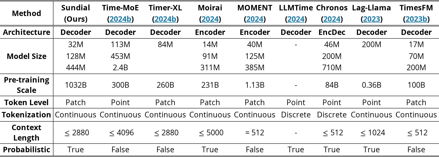
On the FEV leaderboard (Ansari et al., 2024), which consists of short-term forecasting datasets, we train Sundial models by TimeFlow Loss with the prediction length of . For the point forecasting (Wu et al., 2022) and GIFT-Eval (Aksu et al., 2024), which consist of forecasting datasets with a prediction length ranging from to , we train Sundial models by TimeFlow Loss with the prediction length of . For the required prediction length less than the model prediction length, we truncate the output generated by Sundial. For the required length more than the prediction horizon, we conduct rolling forecasting. Following Chronos (Ansari et al., 2024), we sample raw predictions to calculate MASE and WQL on FEV. Being consistent to Moirai (Woo et al., 2024), we sample raw predictions to calculate MASE and CRPS for GIFT-Eval. The sampling step is fixed as . Configurations of Sundial in different sizes are provided in Table 5. We provide a model summary in Table 6, which summarizes several aspects of current time series foundation models.
| Model | Patch Size | Context Length | Prediction Length | Layers | Dimension | MHA Heads | TimeFlow | Total Parameters |
|---|---|---|---|---|---|---|---|---|
| 6 | M | |||||||
| 12 | M | |||||||
| 24 | M |
View original table
| Method | Sundial | Time-MoE | Timer-XL | Moirai | MOMENT | LLMTime | Chronos | Lag-Llama | TimesFM |
|---|---|---|---|---|---|---|---|---|---|
| (Ours) | (2024b) | (2024b) | (2024) | (2024) | (2024) | (2024) | (2023) | (2023b) | |
| Architecture | Decoder | Decoder | Decoder | Encoder | Encoder | Decoder | EncDec | Decoder | Decoder |
| Model Size | 32M | 113M | 84M | 14M | 40M | - | 46M | 200M | 17M |
| 128M | 453M | 91M | 125M | 200M | 70M | ||||
| 444M | 2.4B | 311M | 385M | 710M | 200M | ||||
| Pre-training Scale | 1032B | 300B | 260B | 231B | 1.13B | - | 84B | 0.36B | 100B |
| Token Level | Patch | Point | Patch | Patch | Patch | Point | Point | Point | Patch |
| Tokenization | Continuous | Continuous | Continuous | Continuous | Continuous | Discrete | Discrete | Continuous | Continuous |
| Context Length | 2880 | 4096 | 2880 | 5000 | = 512 | - | 512 | 1024 | 512 |
| Probabilistic | True | False | False | True | False | True | True | True | False |
View original table
Mode collapse is a failure of representation learning, where a model generates a limited variety of outputs, ignoring the diversity in the training data. For time series foundation models, mode collapse stems from the heterogeneity of the time series distribution, e.g., a similar lookback time series goes into divergent trending. In other words, the semantics of time series patterns are highly unstable. It sometimes leads to over-smooth predictions from models optimized by MSE becuase the results are global-optimal for this loss (See showcases on the right of Figure 14-15). Such a training objective pre-defines a unimodal predictive distribution of data, which struggles to accommodate large-scale datasets like TimeBench.
Our work addresses this phenomenon through generative modeling. Generative forecasters learn flexible distributions without relying on probabilistic priors. We evaluate the distributional metric Continuous Ranked Probability Score (CRPS) to assess the quality of generated predictions across different training objectives. The results indicate that the predictive distribution modeled by TimeFlow is more coherent and diverse compared to alternative training objectives, particularly on the highly diverse GIFT-Eval (Aksu et al., 2024). It validates the effectiveness of TimeFlow in mitigating mode collapse.
| Objective | ETTh1 | ETTh2 | ETTm1 | ETTm2 | ECL | Weather | GIFT-Eval |
|---|---|---|---|---|---|---|---|
| TimeFlow Loss | 0.0059 | 0.0037 | 0.0057 | 0.0029 | 0.0082 | 0.0021 | 0.5050 |
| Diffusion Loss | 0.0082 | 0.0053 | 0.0070 | 0.0039 | 0.0095 | 0.0032 | 0.5340 |
| MSE Loss | 0.0063 | 0.0040 | 0.0058 | 0.0032 | 0.0080 | 0.0023 | 0.6420 |
View original table

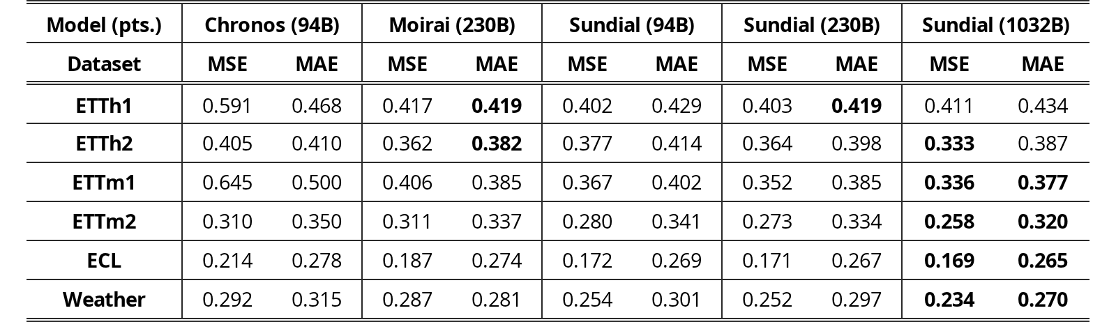
We compare Sundial with other time series foundation models that are pre-trained with smaller datasets: Chronos (Ansari et al., 2024) is pre-trained on 94 billion time points, and Moirai is pre-trained on 230 billion time points. As their pre-training datasets are part of the subset of TimeBench, we also conduct pre-training on Sundial using these subsets. As shown in Table 8, these results highlight the scaling behavior of Sundial using larger datasets. Additionally, Sundial still achieves better zero-shot forecasting than its counterpart models with the same pre-training dataset.
| Model (pts.) | Chronos (94B) | Moirai (230B) | Sundial (94B) | Sundial (230B) | Sundial (1032B) | |||||
|---|---|---|---|---|---|---|---|---|---|---|
| Dataset | MSE | MAE | MSE | MAE | MSE | MAE | MSE | MAE | MSE | MAE |
| ETTh1 | 0.591 | 0.468 | 0.417 | 0.419 | 0.402 | 0.429 | 0.403 | 0.419 | 0.411 | 0.434 |
| ETTh2 | 0.405 | 0.410 | 0.362 | 0.382 | 0.377 | 0.414 | 0.364 | 0.398 | 0.333 | 0.387 |
| ETTm1 | 0.645 | 0.500 | 0.406 | 0.385 | 0.367 | 0.402 | 0.352 | 0.385 | 0.336 | 0.377 |
| ETTm2 | 0.310 | 0.350 | 0.311 | 0.337 | 0.280 | 0.341 | 0.273 | 0.334 | 0.258 | 0.320 |
| ECL | 0.214 | 0.278 | 0.187 | 0.274 | 0.172 | 0.269 | 0.171 | 0.267 | 0.169 | 0.265 |
| Weather | 0.292 | 0.315 | 0.287 | 0.281 | 0.254 | 0.301 | 0.252 | 0.297 | 0.234 | 0.270 |
View original table
Time series foundation models operate independently of training, functioning similarly to statistical methods. Given specific forecasting tasks, one of the most important hyperparameters is the lookback length. Unlike fixed-context models, Sundial offers flexibility for practitioners, allowing the context length to be dynamically adjusted during inference. In Figure 10, we present the performance of Sundial utilizing various lookback lengths. Based on our observations, we contend that performance is largely dependent on the forecasting task itself. Specifically, the size of the lookback window can be tuned to meet the forecasting horizon and data periodicity. Time series foundation models provide a training-free approach for rapid adjustments; still, they should enhance their fundamental long-context capabilities to handle high-frequency data.
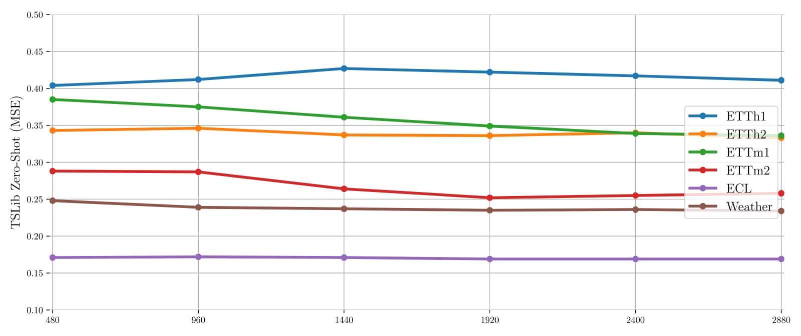
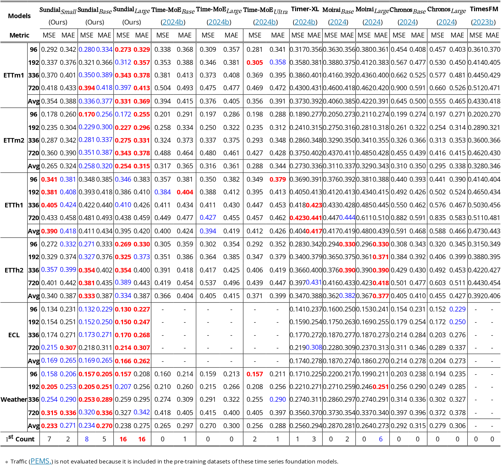
Table 9 provides full zero-shot results on Time-Series-Library forecasting benchmark (Wu et al., 2022), including prediction horizons in . We build Sundial with different model sizes with configurations in Table 5. The context length is fixed as . We truncate the model’s predictions for tasks requiring a prediction length less than .
We compare the most advanced time series foundation models based on their official checkpoints, including Time-MoE (Shi et al., 2024b), Timer (Liu et al., 2024b; Liu et al., 2024c), Moirai (Woo et al., 2024), TimesFM (Das et al., 2023b), and Chronos (Ansari et al., 2024). We conduct zero-shot evaluations on datasets that are not included during the pre-training of the corresponding models. For each of the evaluated model, we use their maximum input length during inference. Metrics (MSE/MAE) are calculated from all predicted windows in the test split of each dataset following Liu et al. (2024b).
We evaluate our models on GIFT-Eval, a benchmark designed to comprehensively assess forecasting performance across diverse time series. GIFT-Eval includes datasets covering time series and million data points, which constitute a total of forecasting configurations. We use the official evaluation suite established by the research team of Salesforce and report aggregated results in Table 2. We evaluate the performance and inference time on the FEV leaderboard, which was originally proposed by Ansari et al. (2024) and established by AutoGluon, which comprises datasets for zero-shot evaluation. We report aggregated metrics in Figure 4 and assess the inference time in Figure 5. We released the detailed results by submitting Sundial to their open benchmark.
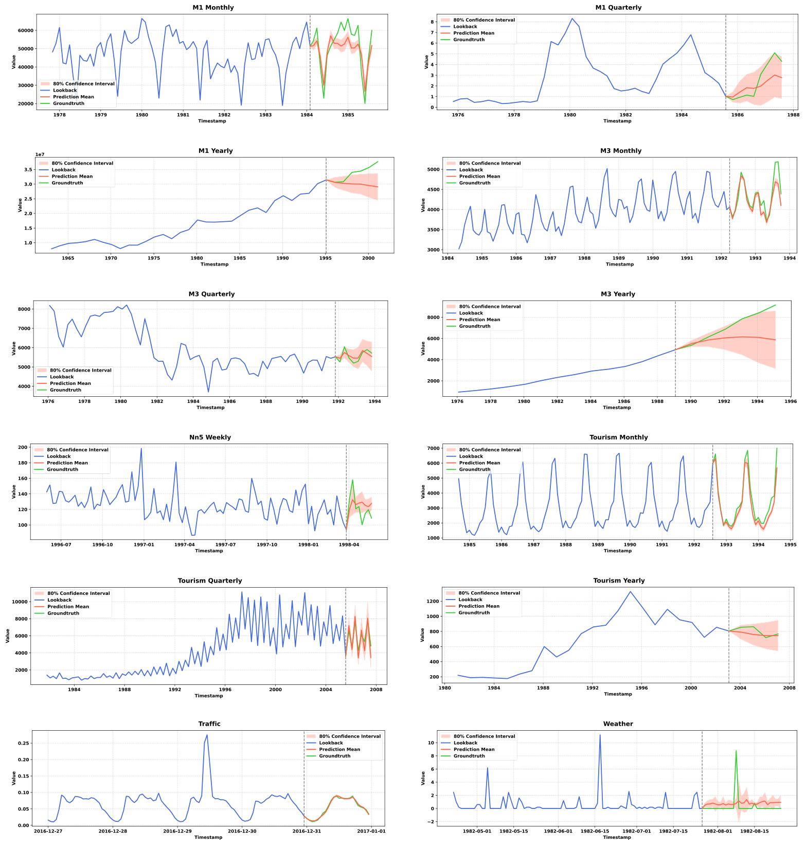
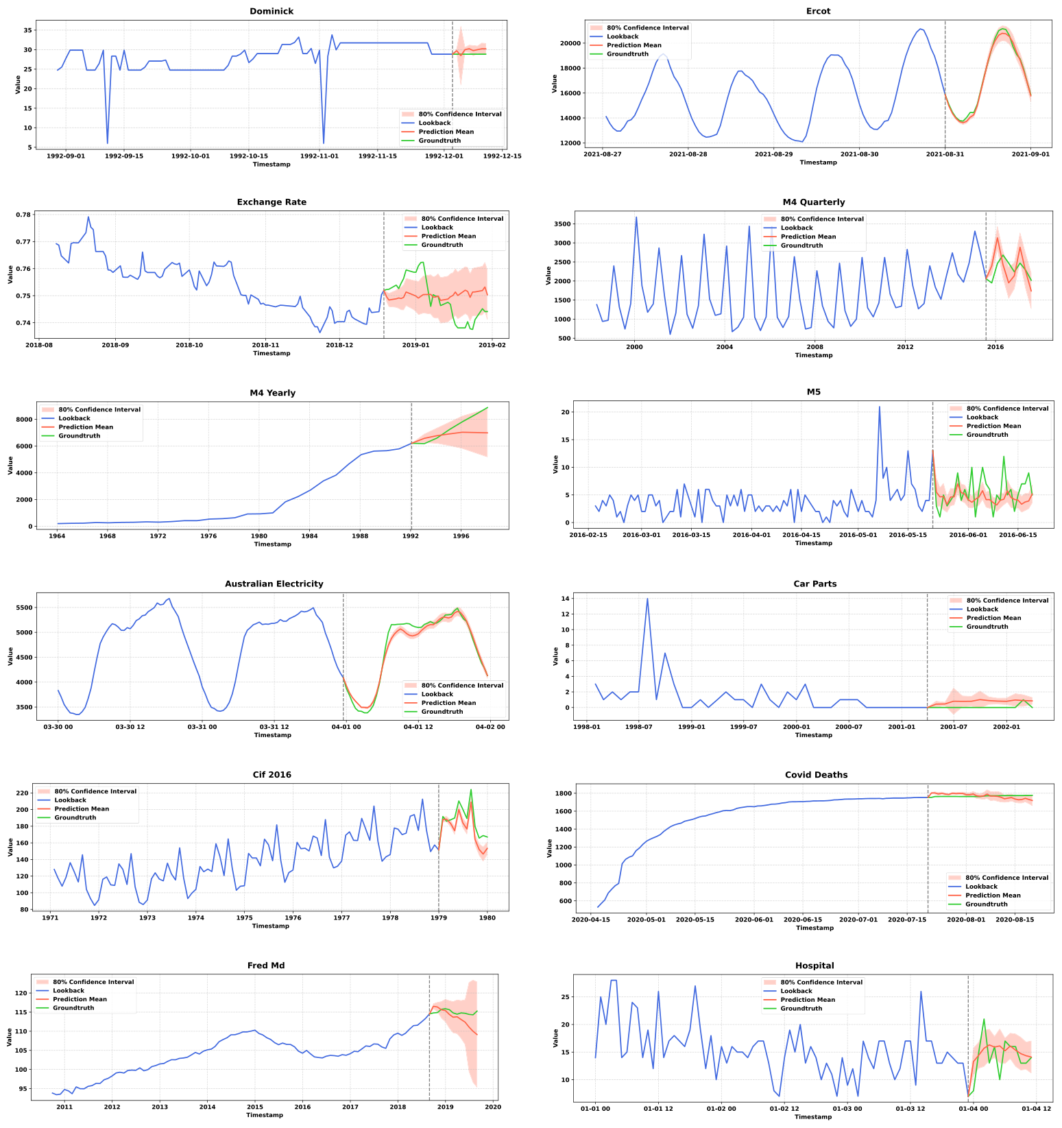
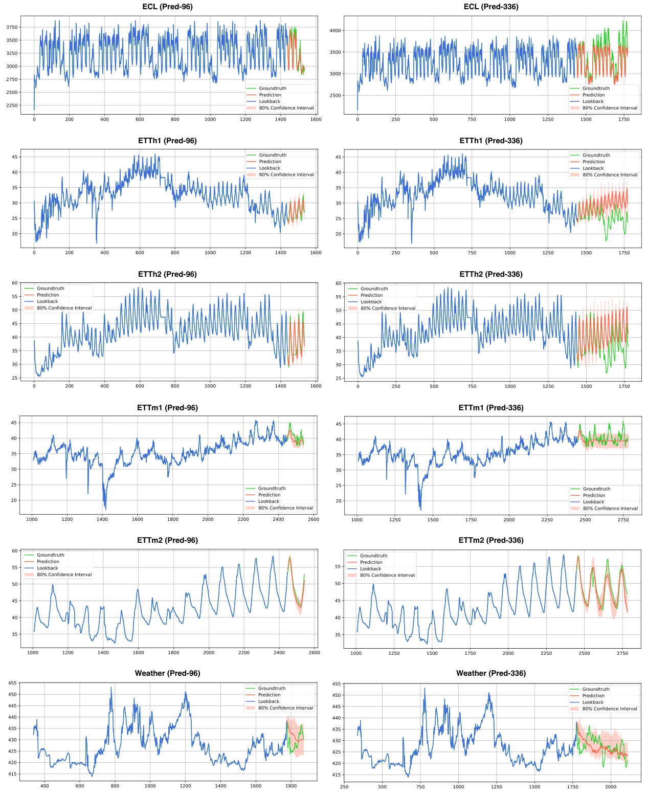
Figure 11-13 present zero-shot forecasting showcases on all the datasets from FEV (Ansari et al., 2024) and TSLib (Wu et al., 2022). By generating predictions with different initial noise, we estimate the median and prediction interval.
| Models | Timer-XL | TimesFM | |||||||||||||||||||||||
|---|---|---|---|---|---|---|---|---|---|---|---|---|---|---|---|---|---|---|---|---|---|---|---|---|---|
| (Ours) | (Ours) | (Ours) | (2024b) | (2024b) | (2024b) | (2024b) | (2024) | (2024) | (2024) | (2024) | (2023b) | ||||||||||||||
| Metric | MSE | MAE | MSE | MAE | MSE | MAE | MSE | MAE | MSE | MAE | MSE | MAE | MSE | MAE | MSE | MAE | MSE | MAE | MSE | MAE | MSE | MAE | MSE | MAE | |
| ETTm1 | 96 | 0.292 | 0.342 | 0.280 | 0.334 | 0.273 | 0.329 | 0.338 | 0.368 | 0.309 | 0.357 | 0.281 | 0.341 | 0.317 | 0.356 | 0.363 | 0.356 | 0.380 | 0.361 | 0.454 | 0.408 | 0.457 | 0.403 | 0.361 | 0.370 |
| 192 | 0.337 | 0.376 | 0.321 | 0.366 | 0.312 | 0.357 | 0.353 | 0.388 | 0.346 | 0.381 | 0.305 | 0.358 | 0.358 | 0.381 | 0.388 | 0.375 | 0.412 | 0.383 | 0.567 | 0.477 | 0.530 | 0.450 | 0.414 | 0.405 | |
| 336 | 0.370 | 0.401 | 0.350 | 0.389 | 0.343 | 0.378 | 0.381 | 0.413 | 0.373 | 0.408 | 0.369 | 0.395 | 0.386 | 0.401 | 0.416 | 0.392 | 0.436 | 0.400 | 0.662 | 0.525 | 0.577 | 0.481 | 0.445 | 0.429 | |
| 720 | 0.418 | 0.433 | 0.394 | 0.418 | 0.397 | 0.413 | 0.504 | 0.493 | 0.475 | 0.477 | 0.469 | 0.472 | 0.430 | 0.431 | 0.460 | 0.418 | 0.462 | 0.420 | 0.900 | 0.591 | 0.660 | 0.526 | 0.512 | 0.471 | |
| Avg | 0.354 | 0.388 | 0.336 | 0.377 | 0.331 | 0.369 | 0.394 | 0.415 | 0.376 | 0.405 | 0.356 | 0.391 | 0.373 | 0.392 | 0.406 | 0.385 | 0.422 | 0.391 | 0.645 | 0.500 | 0.555 | 0.465 | 0.433 | 0.418 | |
| ETTm2 | 96 | 0.178 | 0.260 | 0.170 | 0.256 | 0.172 | 0.255 | 0.201 | 0.291 | 0.197 | 0.286 | 0.198 | 0.288 | 0.189 | 0.277 | 0.205 | 0.273 | 0.211 | 0.274 | 0.199 | 0.274 | 0.197 | 0.271 | 0.202 | 0.270 |
| 192 | 0.235 | 0.304 | 0.229 | 0.300 | 0.227 | 0.296 | 0.258 | 0.334 | 0.250 | 0.322 | 0.235 | 0.312 | 0.241 | 0.315 | 0.275 | 0.316 | 0.281 | 0.318 | 0.261 | 0.322 | 0.254 | 0.314 | 0.289 | 0.321 | |
| 336 | 0.287 | 0.342 | 0.281 | 0.337 | 0.275 | 0.331 | 0.324 | 0.373 | 0.337 | 0.375 | 0.293 | 0.348 | 0.286 | 0.348 | 0.329 | 0.350 | 0.341 | 0.355 | 0.326 | 0.366 | 0.313 | 0.353 | 0.360 | 0.366 | |
| 720 | 0.360 | 0.390 | 0.351 | 0.387 | 0.343 | 0.378 | 0.488 | 0.464 | 0.480 | 0.461 | 0.427 | 0.428 | 0.375 | 0.402 | 0.437 | 0.411 | 0.485 | 0.428 | 0.455 | 0.439 | 0.416 | 0.415 | 0.462 | 0.430 | |
| Avg | 0.265 | 0.324 | 0.258 | 0.320 | 0.254 | 0.315 | 0.317 | 0.365 | 0.316 | 0.361 | 0.288 | 0.344 | 0.273 | 0.336 | 0.311 | 0.337 | 0.329 | 0.343 | 0.310 | 0.350 | 0.295 | 0.338 | 0.328 | 0.346 | |
| ETTh1 | 96 | 0.341 | 0.381 | 0.348 | 0.385 | 0.346 | 0.383 | 0.357 | 0.381 | 0.350 | 0.382 | 0.349 | 0.379 | 0.369 | 0.391 | 0.376 | 0.392 | 0.381 | 0.388 | 0.440 | 0.393 | 0.441 | 0.390 | 0.414 | 0.404 |
| 192 | 0.381 | 0.408 | 0.393 | 0.418 | 0.386 | 0.410 | 0.384 | 0.404 | 0.388 | 0.412 | 0.395 | 0.413 | 0.405 | 0.413 | 0.412 | 0.413 | 0.434 | 0.415 | 0.492 | 0.426 | 0.502 | 0.524 | 0.465 | 0.434 | |
| 336 | 0.405 | 0.424 | 0.422 | 0.440 | 0.410 | 0.426 | 0.411 | 0.434 | 0.411 | 0.430 | 0.447 | 0.453 | 0.418 | 0.423 | 0.433 | 0.428 | 0.485 | 0.445 | 0.550 | 0.462 | 0.576 | 0.467 | 0.503 | 0.456 | |
| 720 | 0.433 | 0.458 | 0.481 | 0.493 | 0.438 | 0.459 | 0.449 | 0.477 | 0.427 | 0.455 | 0.457 | 0.462 | 0.423 | 0.441 | 0.447 | 0.444 | 0.611 | 0.510 | 0.882 | 0.591 | 0.835 | 0.583 | 0.511 | 0.481 | |
| Avg | 0.390 | 0.418 | 0.411 | 0.434 | 0.395 | 0.420 | 0.400 | 0.424 | 0.394 | 0.419 | 0.412 | 0.426 | 0.404 | 0.417 | 0.417 | 0.419 | 0.480 | 0.439 | 0.591 | 0.468 | 0.588 | 0.466 | 0.473 | 0.443 | |
| ETTh2 | 96 | 0.272 | 0.332 | 0.271 | 0.333 | 0.269 | 0.330 | 0.305 | 0.359 | 0.302 | 0.354 | 0.292 | 0.352 | 0.283 | 0.342 | 0.294 | 0.330 | 0.296 | 0.330 | 0.308 | 0.343 | 0.320 | 0.345 | 0.315 | 0.349 |
| 192 | 0.329 | 0.374 | 0.327 | 0.376 | 0.325 | 0.373 | 0.351 | 0.386 | 0.364 | 0.385 | 0.347 | 0.379 | 0.340 | 0.379 | 0.365 | 0.375 | 0.361 | 0.371 | 0.384 | 0.392 | 0.406 | 0.399 | 0.388 | 0.395 | |
| 336 | 0.357 | 0.399 | 0.354 | 0.402 | 0.354 | 0.400 | 0.391 | 0.418 | 0.417 | 0.425 | 0.406 | 0.419 | 0.366 | 0.400 | 0.376 | 0.390 | 0.390 | 0.390 | 0.429 | 0.430 | 0.492 | 0.453 | 0.422 | 0.427 | |
| 720 | 0.401 | 0.442 | 0.381 | 0.435 | 0.389 | 0.443 | 0.419 | 0.454 | 0.537 | 0.496 | 0.439 | 0.447 | 0.397 | 0.431 | 0.416 | 0.433 | 0.423 | 0.418 | 0.501 | 0.477 | 0.603 | 0.511 | 0.443 | 0.454 | |
| Avg | 0.340 | 0.387 | 0.333 | 0.387 | 0.334 | 0.387 | 0.366 | 0.404 | 0.405 | 0.415 | 0.371 | 0.399 | 0.347 | 0.388 | 0.362 | 0.382 | 0.367 | 0.377 | 0.405 | 0.410 | 0.455 | 0.427 | 0.392 | 0.406 | |
| ECL | 96 | 0.134 | 0.231 | 0.132 | 0.229 | 0.130 | 0.227 | - | - | - | - | - | - | 0.141 | 0.237 | 0.160 | 0.250 | 0.153 | 0.241 | 0.154 | 0.231 | 0.152 | 0.229 | - | - |
| 192 | 0.154 | 0.251 | 0.152 | 0.250 | 0.150 | 0.247 | - | - | - | - | - | - | 0.159 | 0.254 | 0.175 | 0.263 | 0.169 | 0.255 | 0.179 | 0.254 | 0.172 | 0.250 | - | - | |
| 336 | 0.174 | 0.271 | 0.173 | 0.271 | 0.170 | 0.268 | - | - | - | - | - | - | 0.177 | 0.272 | 0.187 | 0.277 | 0.187 | 0.273 | 0.214 | 0.284 | 0.203 | 0.276 | - | - | |
| 720 | 0.215 | 0.307 | 0.218 | 0.311 | 0.214 | 0.307 | - | - | - | - | - | - | 0.219 | 0.308 | 0.228 | 0.309 | 0.237 | 0.313 | 0.311 | 0.346 | 0.289 | 0.337 | - | - | |
| Avg | 0.169 | 0.265 | 0.169 | 0.265 | 0.166 | 0.262 | - | - | - | - | - | - | 0.174 | 0.278 | 0.187 | 0.274 | 0.186 | 0.270 | 0.214 | 0.278 | 0.204 | 0.273 | - | - | |
| Weather | 96 | 0.158 | 0.206 | 0.157 | 0.205 | 0.157 | 0.208 | 0.160 | 0.214 | 0.159 | 0.213 | 0.157 | 0.211 | 0.171 | 0.225 | 0.220 | 0.217 | 0.199 | 0.211 | 0.203 | 0.238 | 0.194 | 0.235 | - | - |
| 192 | 0.205 | 0.253 | 0.205 | 0.251 | 0.207 | 0.256 | 0.210 | 0.260 | 0.215 | 0.266 | 0.208 | 0.256 | 0.221 | 0.271 | 0.271 | 0.259 | 0.246 | 0.251 | 0.256 | 0.290 | 0.249 | 0.285 | - | - | |
| 336 | 0.254 | 0.290 | 0.253 | 0.289 | 0.259 | 0.295 | 0.274 | 0.309 | 0.291 | 0.322 | 0.255 | 0.290 | 0.274 | 0.311 | 0.286 | 0.297 | 0.274 | 0.291 | 0.314 | 0.336 | 0.302 | 0.327 | - | - | |
| 720 | 0.315 | 0.336 | 0.320 | 0.336 | 0.327 | 0.342 | 0.418 | 0.405 | 0.415 | 0.400 | 0.405 | 0.397 | 0.356 | 0.370 | 0.373 | 0.354 | 0.337 | 0.340 | 0.397 | 0.396 | 0.372 | 0.378 | - | - | |
| Avg | 0.233 | 0.271 | 0.234 | 0.270 | 0.238 | 0.275 | 0.265 | 0.297 | 0.270 | 0.300 | 0.256 | 0.288 | 0.256 | 0.294 | 0.287 | 0.281 | 0.264 | 0.273 | 0.292 | 0.315 | 0.279 | 0.306 | - | - | |
| Count | 7 | 2 | 8 | 5 | 16 | 16 | 0 | 1 | 0 | 0 | 2 | 1 | 1 | 3 | 0 | 2 | 0 | 6 | 0 | 0 | 0 | 0 | 0 | 0 | |
View original table
As we introduce generative modeling in time series foundation models, we compare zero-shot forecasting showcases from two types of models, including (1) Sundial, a generative forecaster pre-trained by TimeFlow, which can predict multiple future possibilities based on a lookback series. (2) Using the same backbone and TimeBench, a Transformer pre-trained by MSE Loss. As a deterministic forecaster, the model can only output the mean prediction. As depicted in Figure 14-15, the unimodal Gaussian prior specified by MSE can be infeasible to handle large-scale pre-training, manifested as sometimes over-smooth predictions in downstream forecasting tasks. Therefore, we hope this work can inspire future paradigms for pre-training time series foundation models and enhance their applicability to real-world scenarios.
Our models represent an initial effort to incorporate generative modeling into time series foundation models, which enables pre-training on heterogeneous time series without specifying any prior distribution. This approach mitigates mode collapse in representation learning and generates a diverse range of probable predictions compared to previous deterministic forecasters. Despite significant progress in enlarging model capacity, the Sundial family may still face hallucinations. The performance on very high-frequency data is not guaranteed, since TimeBench contains many middle- and low-frequency time series. Therefore, an important future direction is to generalize Sundial to multi-scale time series. This situation may also indicate new opportunities during inference. As we only adopt a naïve sampling strategy that begins with random Gaussian noise, it leaves much room for future improvement in sampling strategy and post-processing, such as frequency normalization.
Another aspect of future development lies in model adaptation. Sundial is pre-trained in a univariate approach to address the discrepancy in variate numbers, which prevents it from explicitly utilizing variate correlations or covariate information. As an increasing number of studies address 2D dimensionality, multivariate pre-training is likely to be conducted for domain-specific time series foundation models. Lastly, while autoregressive models provide flexibility in the input context length, multiple steps of autoregression may still lead to over-smooth predictions and unreliable results.
In this work, we present Sundial, a family of time series foundation models to facilitate out-of-the-box forecasting. Our models employ native tokenization for continuous-valued time series and incorporate a flexible training objective, proposed as TimeFlow Loss, to enable probabilistic forecasting. With an unprecedented model capacity and a trillion-scale dataset, our models can be used directly or adapted for various forecasting scenarios, such as energy planning, weather forecasting, and financial risk prevention. With multiple predictions generation and a just-in-time inference speed, our model enhances the reliability of decision-making and streamlines the forecasting pipeline for practitioners. This paper primarily focuses on scientific research and does not present any evident negative social impact.
We curate TimeBench, a trillion-level time series dataset for pre-training foundation models for time series analysis, which we believe will be beneficial to the research community. Technically, we propose a TimeFlow Loss to facilitate the learning of flexible next-patch distributions. Conditioned on the lookback representations acquired by autoregressive Transformers, our model is endowed with a novel generative capability for probabilistic forecasting, enhancing representation learning of Transformers without the need for discrete tokenization. Through pre-training on an unprecedented scale, we identify subtle scalability bottlenecks that are not solely attributable to architectural design but are predominantly influenced by the training objectives of foundation models. The proposed TimeFlow Loss applied to autoregressive and generative models may provide insights for the future development of time series foundation models.