MARS: Modular Agent with Reflective Search for Automated AI Research
arXiv:2602.02660v3 · This workspace stays on this version. Check arXiv for newer versions
Some source details need review 29 to check
Original formulas, table values and figures are preserved. Comparison can miss differences; use the original PDF to check details.
Reading view checked: 234 math expressions, 0 rendering failures; 45 of 45 images available.
Compared 166 of 174 source passages against 44 of 66 PDF pages.
The HTML source contains failed formatting commands; these were omitted from the reading view. The original sources are retained. (1)
- Some graphics are laid out differently in the HTML source than in the paper (text or formulas outside their frame); check the original PDF. (27)
- A8_p2_pic1: the arXiv HTML draws text or formulas of this graphic outside its frame and it could not be corrected safely (too-small); the image shows the HTML layout, which differs from the PDF.
- A8_p3_pic1: the arXiv HTML draws text or formulas of this graphic outside its frame and it could not be corrected safely (too-small); the image shows the HTML layout, which differs from the PDF.
- A8_p4_pic1: the arXiv HTML draws text or formulas of this graphic outside its frame and it could not be corrected safely (too-small); the image shows the HTML layout, which differs from the PDF.
- A8_p5_pic1: the arXiv HTML draws text or formulas of this graphic outside its frame and it could not be corrected safely (too-small); the image shows the HTML layout, which differs from the PDF.
- A8_p6_pic1: the arXiv HTML draws text or formulas of this graphic outside its frame and it could not be corrected safely (too-small); the image shows the HTML layout, which differs from the PDF.
- A8_p7_pic1: the arXiv HTML draws text or formulas of this graphic outside its frame and it could not be corrected safely (too-small); the image shows the HTML layout, which differs from the PDF.
- A8_p8_pic1: the arXiv HTML draws text or formulas of this graphic outside its frame and it could not be corrected safely (too-small); the image shows the HTML layout, which differs from the PDF.
- A8_p9_pic1: the arXiv HTML draws text or formulas of this graphic outside its frame and it could not be corrected safely (too-small); the image shows the HTML layout, which differs from the PDF.
- A8_p10_pic1: the arXiv HTML draws text or formulas of this graphic outside its frame and it could not be corrected safely (too-small); the image shows the HTML layout, which differs from the PDF.
- A8_p11_pic1: the arXiv HTML draws text or formulas of this graphic outside its frame and it could not be corrected safely (too-small); the image shows the HTML layout, which differs from the PDF.
- A8_p12_pic1: the arXiv HTML draws text or formulas of this graphic outside its frame and it could not be corrected safely (too-small); the image shows the HTML layout, which differs from the PDF.
- A8_p13_pic1: the arXiv HTML draws text or formulas of this graphic outside its frame and it could not be corrected safely (too-small); the image shows the HTML layout, which differs from the PDF.
- A8_p14_pic1: the arXiv HTML draws text or formulas of this graphic outside its frame and it could not be corrected safely (too-small); the image shows the HTML layout, which differs from the PDF.
- A8_p15_pic1: the arXiv HTML draws text or formulas of this graphic outside its frame and it could not be corrected safely (too-small); the image shows the HTML layout, which differs from the PDF.
- A8_p16_pic1: the arXiv HTML draws text or formulas of this graphic outside its frame and it could not be corrected safely (too-small); the image shows the HTML layout, which differs from the PDF.
- A8_p17_pic1: the arXiv HTML draws text or formulas of this graphic outside its frame and it could not be corrected safely (too-small); the image shows the HTML layout, which differs from the PDF.
- A8_p18_pic1: the arXiv HTML draws text or formulas of this graphic outside its frame and it could not be corrected safely (too-small); the image shows the HTML layout, which differs from the PDF.
- A8_p19_pic1: the arXiv HTML draws text or formulas of this graphic outside its frame and it could not be corrected safely (too-small); the image shows the HTML layout, which differs from the PDF.
- A8_p20_pic1: the arXiv HTML draws text or formulas of this graphic outside its frame and it could not be corrected safely (too-small); the image shows the HTML layout, which differs from the PDF.
- A9_p2_pic1: the arXiv HTML draws text or formulas of this graphic outside its frame and it could not be corrected safely (too-small); the image shows the HTML layout, which differs from the PDF.
- A9_p3_pic1: the arXiv HTML draws text or formulas of this graphic outside its frame and it could not be corrected safely (too-small); the image shows the HTML layout, which differs from the PDF.
- A9_p4_pic1: the arXiv HTML draws text or formulas of this graphic outside its frame and it could not be corrected safely (too-small); the image shows the HTML layout, which differs from the PDF.
- A9_p5_pic1: the arXiv HTML draws text or formulas of this graphic outside its frame and it could not be corrected safely (too-small); the image shows the HTML layout, which differs from the PDF.
- A9_p6_pic1: the arXiv HTML draws text or formulas of this graphic outside its frame and it could not be corrected safely (too-small); the image shows the HTML layout, which differs from the PDF.
- A9_p7_pic1: the arXiv HTML draws text or formulas of this graphic outside its frame and it could not be corrected safely (too-small); the image shows the HTML layout, which differs from the PDF.
- A9_p8_pic1: the arXiv HTML draws text or formulas of this graphic outside its frame and it could not be corrected safely (too-small); the image shows the HTML layout, which differs from the PDF.
- A9_p9_pic1: the arXiv HTML draws text or formulas of this graphic outside its frame and it could not be corrected safely (too-small); the image shows the HTML layout, which differs from the PDF.
- This long paper was only partially compared; the original sources remain available.
45 of 45 figure, table and graphic images captured. Open original PDF
Abstract
A critical bottleneck in automating AI research is the execution of complex machine learning engineering (MLE) tasks. MLE differs from general software engineering due to computationally expensive evaluation (e.g., model training) and opaque performance attribution. Current LLM-based agents struggle here, often generating monolithic scripts that ignore execution costs and causal factors. We introduce MARS (Modular Agent with Reflective Search), a framework optimized for autonomous AI research. MARS relies on three pillars: (1) Budget-Aware Planning via cost-constrained Monte Carlo Tree Search (MCTS) to explicitly balance performance with execution expense; (2) Modular Construction, employing a “Design-Decompose-Implement” pipeline to manage complex research repositories; and (3) Comparative Reflective Memory, which addresses credit assignment by analyzing solution differences to distill high-signal insights. MARS achieves state-of-the-art performance among open-source frameworks on MLE-Bench under comparable settings, maintaining competitiveness with the global leaderboard’s top methods. Furthermore, the system exhibits qualitative “Aha!” moments, where 63% of all utilized lessons originate from cross-branch transfer, demonstrating that the agent effectively generalizes insights across search paths.
The integration of Large Language Models (LLMs) into software engineering has fundamentally transformed code generation, evolving from simple auto-completion to autonomous agents capable of resolving GitHub issues Jimenez et al. (2023); Yang et al. (2024) and generating functional scripts (Li et al., 2022; Wang et al., 2025; Jiang et al., 2025). However, while current agents excel at general software maintenance tasks – such as patching bugs or writing unit tests – they face significant hurdles when applied to the domain of Automating AI Research (Chan et al., 2025; Tian et al., 2024; Wijk et al., 2025; Yamada et al., 2025; Starace et al., 2025). A critical bottleneck in this domain is the execution of complex machine learning engineering (MLE) tasks. Unlike standard software development, where correctness is often binary and verification is computationally cheap, MLE is a probabilistic, resource-intensive endeavor. It requires not only coding intelligence but also the strategic foresight to navigate a landscape defined by computationally expensive evaluations, opaque performance attribution, and high architectural complexity.
Existing agentic frameworks, designed primarily for monolithic code generation, struggle to adapt to these constraints. First, they typically view problem-solving as a purely code-based challenge (Huang et al., 2024; Jiang et al., 2025; Toledo et al., 2026), ignoring the economic reality of research: model training and data processing consume vast computational resources. An agent that improves model accuracy by 0.1% but increases training time from one hour to ten hours is often practically useless, yet standard search algorithms would prioritize it. Second, the monolithic and unstructured scripts often produced by previous LLM agents are fragile and ill-suited for the modular complexity required in research repositories, where data loading, model architecture, and training loops must interact seamlessly. Finally, research progress is iterative and opaque; when a new experiment yields better results, it is difficult to isolate the causal factor. Standard memory-based agents (Packer et al., 2023; Shinn et al., 2023; Xu et al., 2026; Ouyang et al., 2026) lack the mechanism to solve this credit assignment problem, often failing to learn effectively from past trials.
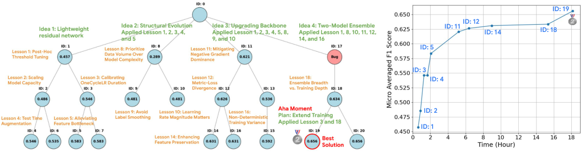
To bridge this gap, we introduce MARS (Modular Agent with Reflective Search), a framework explicitly optimized for the distinct constraints of autonomous scientific discovery. MARS reformulates the research process as a search for an optimal software repository, governed by three core pillars. To address the high cost of evaluation, we employ Budget-Aware Planning via a cost-constrained Monte Carlo Tree Search (MCTS). Unlike general search algorithms, our method explicitly balances performance maximization with execution expense, prioritizing efficient solutions – such as favoring a 1-hour training run over a 4-hour run if performance is comparable – to optimize the discovery rate within a fixed budget. To manage architectural complexity, we replace fragile scripting with a Modular “Design-Decompose-Implement” pipeline. This structure employs specialized agents to architect solutions into independent, testable modules. Finally, to resolve the credit assignment problem, we introduce Comparative Reflective Memory. By analyzing the differences between the current solution and the best-known solution, the agent distills high-signal, causal insights, isolating the specific factors driving performance shifts in a way that standard memory mechanisms cannot. As illustrated in Figure 1, these pillars allow MARS to experience “Aha!” moments during long-horizon exploration, successfully navigating complex optimization landscapes where baselines fail.
Our contributions are summarized as follows:
- •
We introduce MARS, a framework aimed at automating AI research by optimizing for complex MLE tasks, featuring a novel combination of Budget-Aware MCTS, a modular implementation pipeline, and Comparative Reflective Memory.
- •
We perform extensive evaluation on the MLE-Bench benchmark, where MARS achieves state-of-the-art performance among open-source frameworks under comparable settings. Ablation studies further validate the necessity of each proposed mechanism.
- •
We provide qualitative analyses of how MARS drives long-horizon exploration. To facilitate future research, we release prompts in Appendix H, and MARS generated code, trajectories in https://github.com/jfc43/MARS.
Recent advancements in LLMs have driven ambitious efforts to automate complex, long-horizon AI research (Lu et al., 2024; Yamada et al., 2025; Weng et al., 2025; Tang et al., 2026; Schmidgall et al., 2025; Pu et al., 2025; Starace et al., 2025). Central to these efforts is the realization that Machine Learning Engineering (MLE) serves as a critical execution bottleneck (Chan et al., 2025; Wijk et al., 2025); without robust autonomous MLE capabilities, higher-level research automation cannot succeed. While numerous agentic frameworks have been proposed to address these challenges (Jiang et al., 2025; Toledo et al., 2026; Yang et al., 2025; Liu et al., 2025b; Team et al., 2025; Li et al., 2025; Nam et al., 2026; Zhu et al., 2026), existing systems predominantly operate under a monolithic paradigm, generating expansive, single-file scripts. This approach typically results in fragile codebases that lack the modularity essential for rigorous engineering. MARS departs from this by enforcing a repository-level paradigm that systematically decomposes tasks into distinct, testable, and maintainable modules, mirroring the professional software architecture required for scalable AI research.
Search Algorithms in Code Generation. Solving long-horizon AI research problems, where code execution is resource-intensive, necessitates effective search strategies for code optimization. While various algorithms have been adapted for these systems – including greedy search (Jiang et al., 2025), Monte Carlo Tree Search (MCTS) (Kocsis and Szepesvári, 2006; Liu et al., 2025b), and Evolutionary search (Team et al., 2025) – they typically optimize solely for task performance, neglecting computational cost. While recent work has introduced “budget awareness” for tool-augmented agents via external plug-ins (Liu et al., 2025a), such methods are primarily designed for discrete actions like web search. In contrast, we introduce Budget-aware MCTS, which integrates an efficiency-guided reward function directly into the search tree. This allows MARS to balance the exploitation of high-performing strategies with the exploration of novel ideas, penalizing computationally expensive solutions to ensure both performance and efficiency.
Reflective Learning and Memory. Enabling agents to improve iteratively through environmental interaction is a rapidly evolving research area. Early approaches, such as Reflexion (Shinn et al., 2023), focus on self-correction using verbal reinforcement derived from prior mistakes. Recently, the field has expanded to include sophisticated memory and distillation frameworks. For instance, several works explore advanced memory architectures for personalization and associative retrieval Tan et al. (2025); Xu et al. (2026), while others focus on refining process memory and distilling execution traces into stable strategies Forouzandeh et al. (2025); Ouyang et al. (2026); Zhu et al. (2026). Closer to our domain, Zhao et al. identify “good practices” by comparing high-level action trajectories, and Jansen et al. cache useful code blocks for future reuse. MARS advances this paradigm by introducing “Lesson Learning”. Unlike prior methods that summarize execution logs to debug errors or track binary success-failure trajectories, our method explicitly analyzes the causal link between code changes and performance variations. This comparative analysis isolates effective algorithmic changes from confounding factors, distilling high-value insights into a lesson pool to guide future exploration.
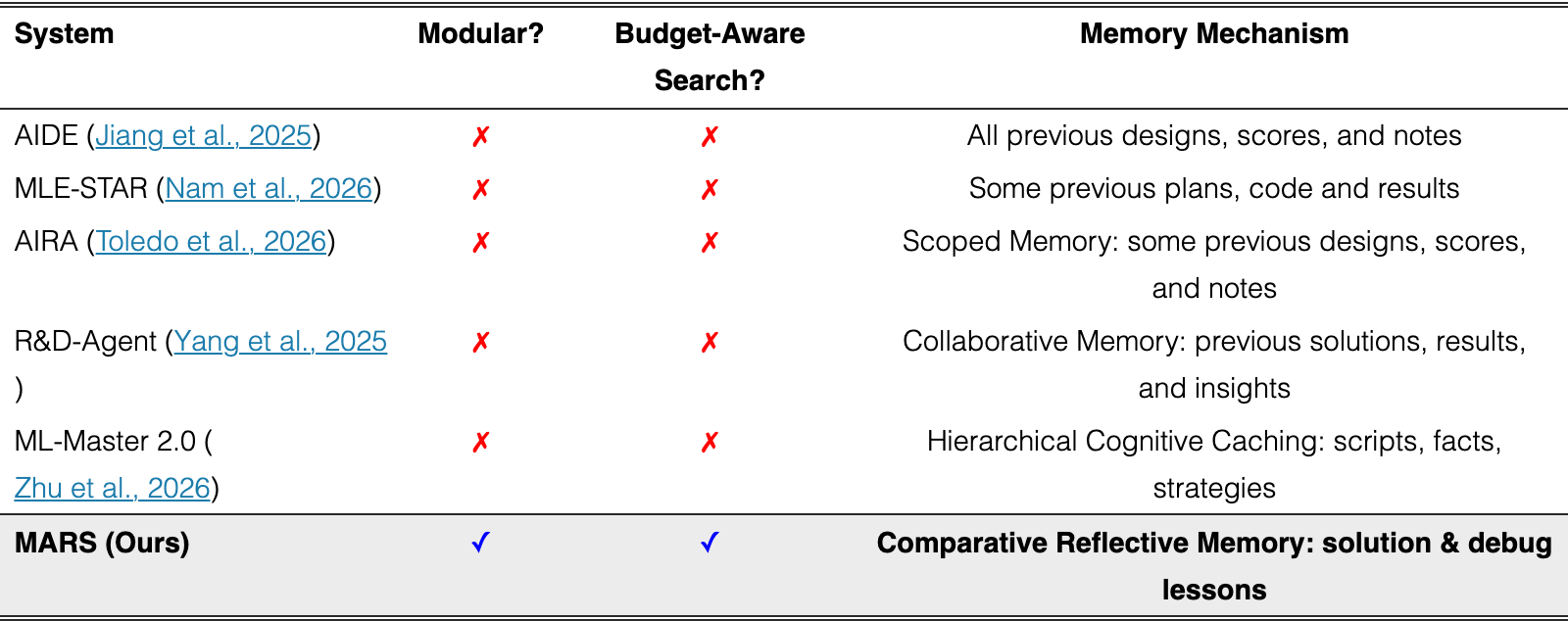
Table 1 summarizes the key differences between MARS and existing MLE agent frameworks.
We first formalize the general problem of Long-Horizon Agentic Problem Solving, where an autonomous agent is tasked with constructing a complex artifacts (e.g., a software system) to satisfy a set of requirements within a constrained budget. Let denote a problem instance defined by the tuple , where: (1) represents the Instruction or requirements provided in natural language. (2) denotes the Environment with which the agent interacts to validate its solutions. This can be a compiler, a simulator, or a dataset depending on the task scenario. (3) is the Objective function that quantifies the quality of the solution.
The goal is to find a solution that maximizes by interacting with , subject to a cost constraint (e.g., time budget or monetary cost):
where the search space for is often vast and unstructured (e.g., the space of all possible Python programs).
Machine Learning Engineering (MLE) is a representative and challenging instantiation of this general problem class. MLE requires the agent to engineer a full pipeline that processes data, trains models, and validates results. In this scenario, consists of the provided datasets while is the performance metric (e.g. accuracy) on the held-out test set. Refer to Appendix B for details.
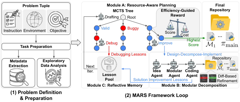
We propose MARS, a general agent scaffolding framework designed to enable autonomous agents to solve long-horizon AI Research problems, as illustrated in Figure 2. Formally, we define the problem as a tuple , where the agent must follow the instruction within an environment to maximize an objective under a cost budget . To address the core challenges of exploration complexity, context management, and solution robustness in this setting, our framework integrates three key capabilities:
- •
Modular Construction Strategy: Instead of generating monolithic scripts, we enforce a structured, repository-level software architecture. This paradigm allows for handing complex logic with greater accuracy, efficient code reuse, and improving testability.
- •
Comparative Reflective Memory: To overcome context window limitations, we introduce a “Lesson Learning” mechanism that distills high-value, causal insights from past interactions (both successes and failures) into a compact, retrievable knowledge base.
- •
Resource-Aware Planning: We employ a budget-aware Monte Carlo Tree Search (MCTS) algorithm to systematically explore the solution space. This allows the system to balance the exploitation of promising candidates with the exploration of novel ideas, preventing local optima, and penalize solutions that are costly.
A primary contribution of this work is the strategic shift from generating monolithic scripts to a Modular Implementation paradigm. This paradigm addresses several inherent limitations of LLM-based coding. First, it bypasses token output limits by distributing code across multiple files. Second, it enhances precision; by focusing on smaller logical units, the agent encounters less context noise and can handle complex logic with greater accuracy. Third, it enables efficiency via caching, as validated modules can be reused without regeneration. Finally, it significantly improves testability, as debugging is localized to specific files rather than requiring full-script diagnosis.
We define a node solution as a tuple comprising a set of independent modules and one orchestration script:
Each module encapsulates a specific sub-task (e.g., data preprocessing, configuration), while the main script orchestrates the end-to-end pipeline.
To instantiate this structure, we employ a three-stage “Design-Decompose-Implement” workflow:
- •
Idea Generation: An Idea Generation Agent articulates a comprehensive natural language plan covering various aspects of the solution.
- •
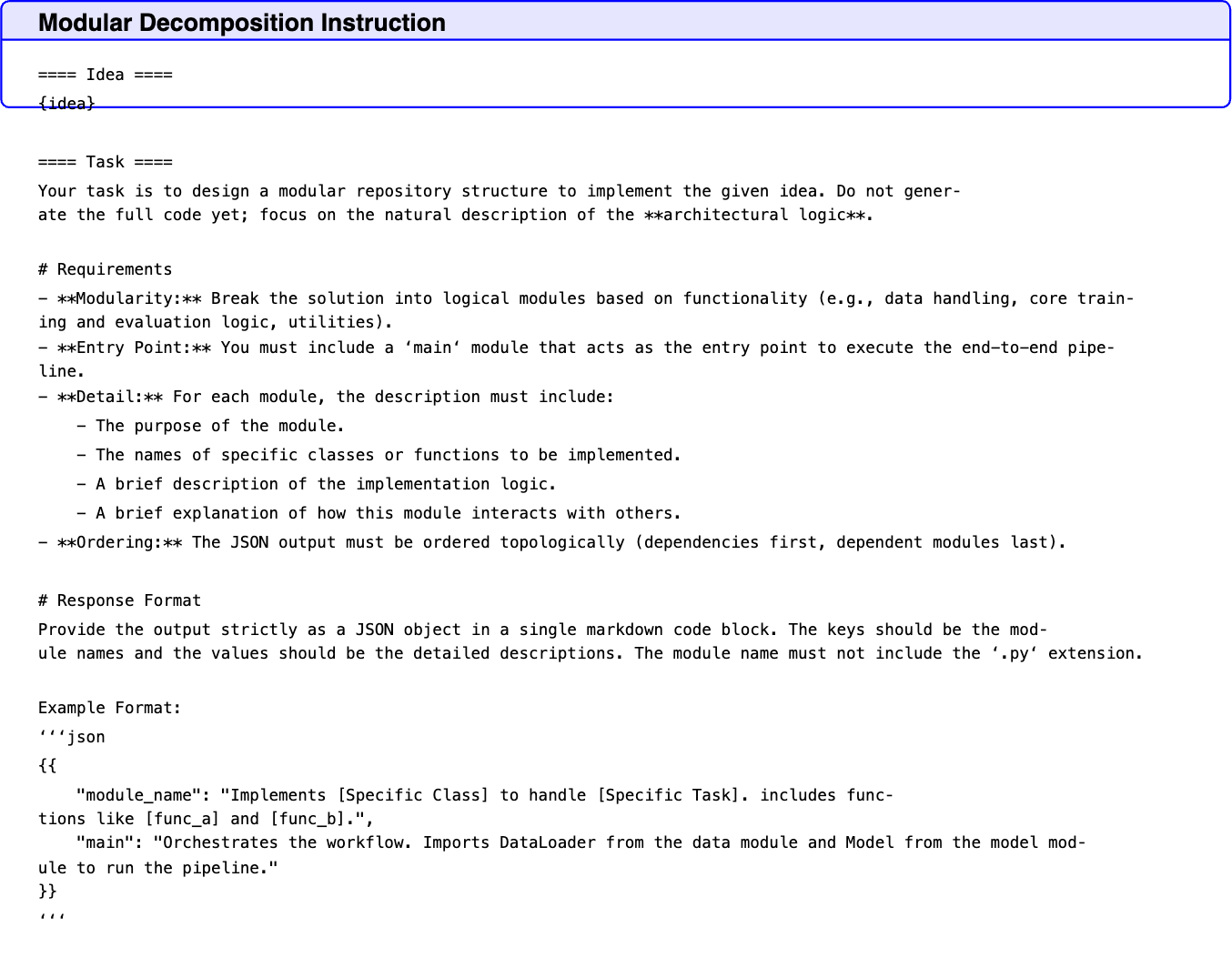
Module Decomposition: A Modular Agent parses the plan and decomposes the solution into logical, independent functional modules.
- •
Component Implementation and Debugging: A Coding Agent sequentially implements each module , employing a validation script to debug and verify functionality. Once validated, the agent orchestrates the modules via the main script .
To prevent wasteful full-repository regeneration, we adopt a Diff-Based Editing mechanism. Code modifications are structured in a standardized diff format, specifying the target file, the block to replace, and the new code. This enables atomic, multi-file updates in a single inference step.
Solving complex tasks requires long-horizon exploration, generating extensive interaction trajectories that often exceed context window constraints. More importantly, research progress is inherently iterative and opaque; when a new experiment yields improved results, isolating the specific causal factors remains a challenge. Standard memory-based agents often lack the mechanisms to solve this credit assignment problem, failing to learn effectively from past trials. To address this, we propose Comparative Reflective Memory, a mechanism designed to distill high-signal, causal insights from the exploration process into a compact lesson pool.
We employ a two-stage process to resolve the credit assignment problem by synthesizing lessons from valid solutions. First, an Empirical Analysis Agent reviews execution logs to extract objective findings (e.g., metric trends). Subsequently, a Lesson Distillation Agent performs a comparative reflection by analyzing the delta between the current solution and the previous best-known solution. This isolates the specific algorithmic changes driving performance shifts, resulting in a structured lesson containing: (1) The isolated causal change, (2) A comparative impact analysis, and (3) A generalized rule for future iterations.
For failed executions, a dedicated agent analyzes the buggy code, error logs, and the applied fix. It outputs a lesson confirming the fix’s efficacy, explaining the failure logic, and providing guidelines to preemptively identify similar errors.
To maintain a high-signal lesson pool, a Review Agent evaluates new lessons against the existing pool through LLM-based reasoning, filtering out redundant insights to ensure the retrieved context remains diverse and relevant.
When executing solution improvement or debugging actions, the agent utilizes relevant knowledge from the corresponding lesson categories. We retain the most recent lessons in the agent’s memory to manage context. To ensure interpretability, the agent is instructed to explicitly cite specific lessons whenever they are applied.
We adopt the Monte Carlo Tree Search (MCTS) framework to explore the solution space, which iterates through four phases: Selection, Expansion, Simulation, and Backpropagation. In this section, we detail our domain-specific modifications: (1) specialized expansion operators, (2) a coherent node selection strategy, and (3) an Efficiency-Guided Reward Function that balances performance with cost. Appendix C provides a review of standard MCTS principles.
We define three distinct operators to transform a parent state into a child solution :
- •
Drafting (Root Expansion): Generates a completely new solution from scratch.
- •
Improvement: Applied to valid, executable nodes. The agent modifies the modules and the main script from to maximize the objective .
- •
Debugging: Applied to nodes where execution failed. The agent inherits the solution structure from but modifies specific modules or the orchestration script to resolve runtime errors. Buggy children enter an automatic debugging loop with up to debugging actions to fix the errors.
We employ the Upper Confidence Bound for Trees (UCT) algorithm to navigate the solution space, balancing the exploitation of high-performing solutions with the exploration of new solutions.
The selection phase begins at the root node. In each step, we select the child node that maximizes the UCT value. This traversal continues recursively until we identify a candidate node, defined as a node that is not yet “fully expanded”.
The root node is set fully expanded unless any of the follow condition occurs: (1) It does not have any children; (2) the best solution has not been improved after implementing valid nodes.
If the traversal reaches a leaf node that is already fully expanded (it implies that no further debugging or improvement is permitted for that branch), then the root node is re-activated to allow for new drafts.
The buggy nodes are always set fully expanded. The valid nodes are set fully expanded if they have children (attempts to improve).
To guide the search efficiently, we design a reward function that rewards performance gains and penalizes long execution time. Let denote the performance metric of a node , and let and represent its execution time and time limit, respectively. We first normalize the performance metric relative to the history of explored nodes . Let and . We define the global normalized score as:
To incorporate budget constraints, we modulate this score by execution latency, defining efficiency-guided reward as:
Where is a penalty weight hyperparameter. A similar function has been proposed in Tan et al. (2019).
While MARS is a general framework, its application requires task-specific components. For Machine Learning Engineering (MLE) tasks, we integrate the following:
Task preparation. We employ a multi-agent system to extract task metadata, formalizing the optimization objective and preparing training, validation, and test datasets.
Data analysis. We employ an agent to perform Exploratory Data Analysis (EDA) to generate a report that guides downstream feature engineering.
Curriculum-Based Exploration. We implement a curriculum-based idea generation strategy that progressively explores simple baselines to complex methods.
Refer to the Appendix D for the details.
Datasets. We evaluate our agent on MLE-Bench (Chan et al., 2025), which consists of 75 challenging competitions from Kaggle, forming a diverse collection of tasks covering natural language processing, computer vision, and tabular data analysis.
Environments. We adhere to the standard MLE-Bench protocol, where agents are allocated a strict 24-hour wall-clock time budget per competition. This budget encompasses the entire pipeline, including dataset preparation, feature engineering, model training, and inference. The experiment for each agent on each competition is conducted on a standard node equipped with one NVIDIA A100 GPU (40GB), 12 vCPUs, 220 GB of RAM, and 1 TB of SSD storage. This setup simulates a realistic, resource-constrained machine learning engineering environment.
Baselines. We compare our method to the agents in the MLE-Bench leaderboard and two state-of-the-art open-source agents: AIDE (Jiang et al., 2025) and AIRA (Toledo et al., 2026). For open-source baselines, we ensure a strictly fair comparison by running them under identical environment configurations and using the same underlying LLMs.
Metrics. Following the standard MLE-Bench evaluation protocol, we report the mean and standard error of the mean (SEM) across three independent runs. Our evaluation focuses on three primary metrics: Above Median Rate (percentage of runs outperforming the median participant), Any Medal Rate (percentage achieving at least a Bronze medal), and Gold Medal Rate (percentage securing a Gold medal).
Hyperparameters. We set the maximum number of lessons in the agent’s memory to to maintain relevant context without context window overflow. We allow up to debugging actions per failure to resolve runtime errors effectively. The branching factor for valid nodes is set to , balancing exploration breadth with depth. We set in the reward function (4) following Tan et al. (2019) to penalize excessive execution time.
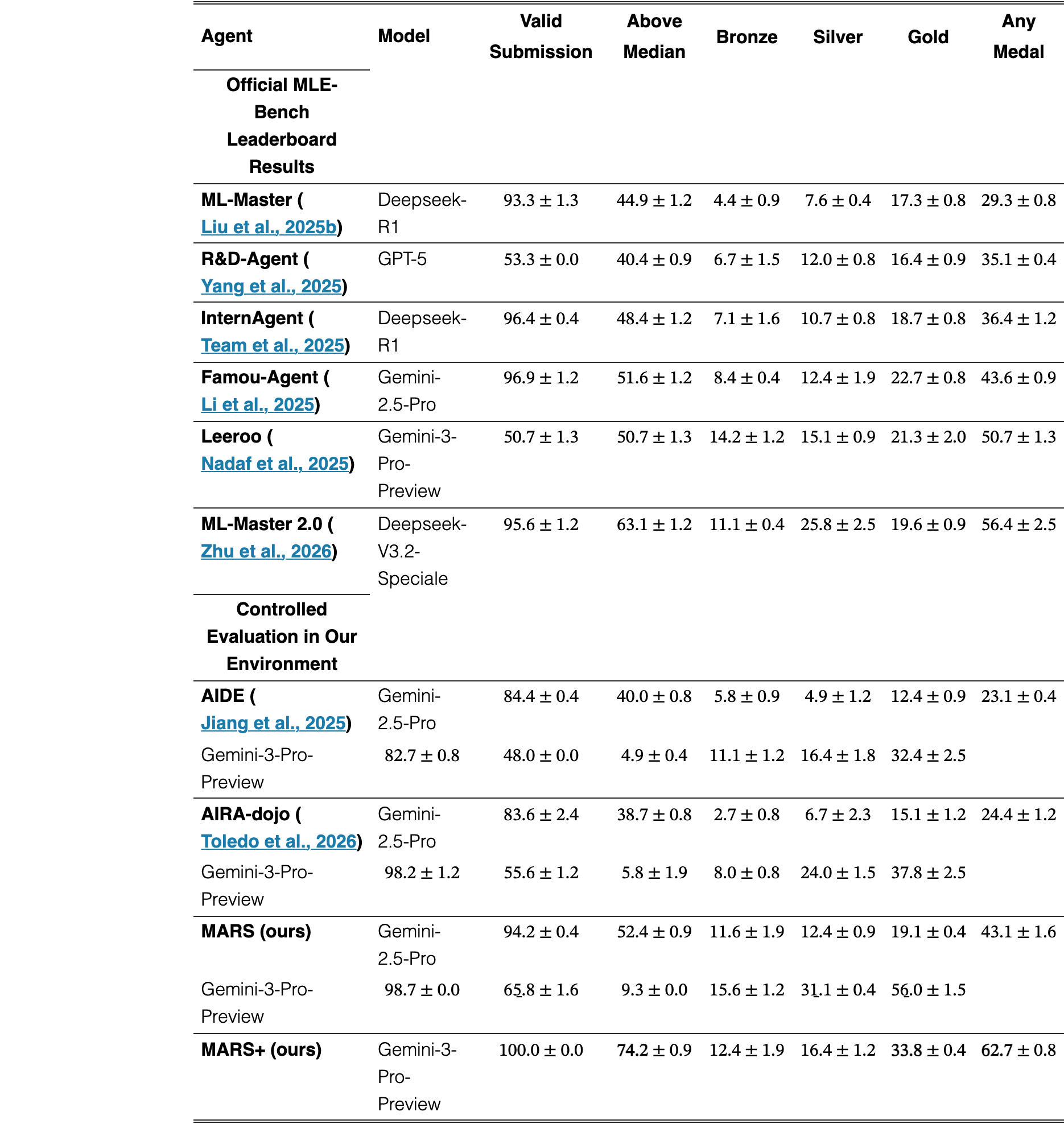
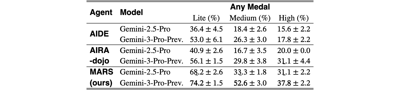
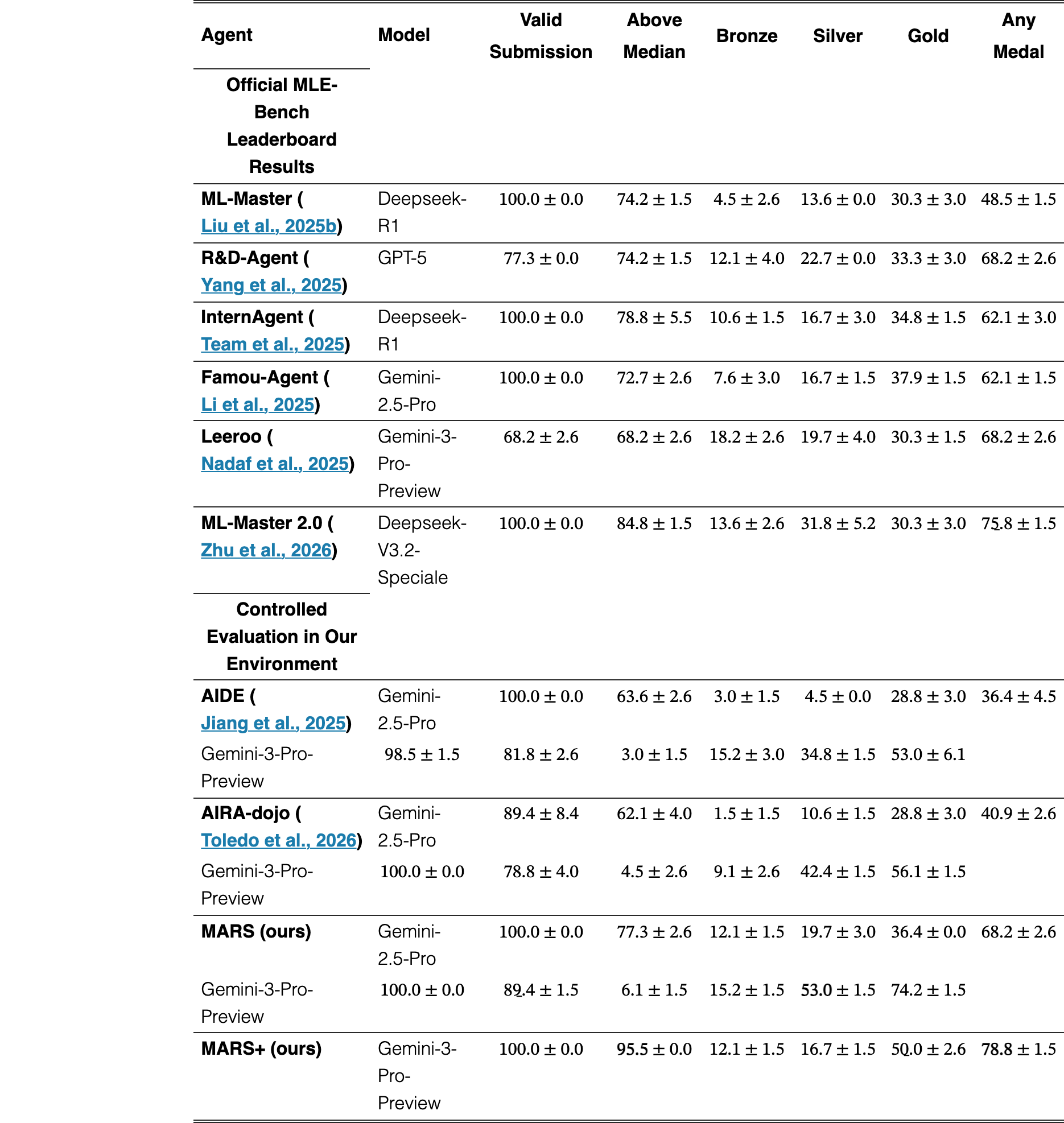
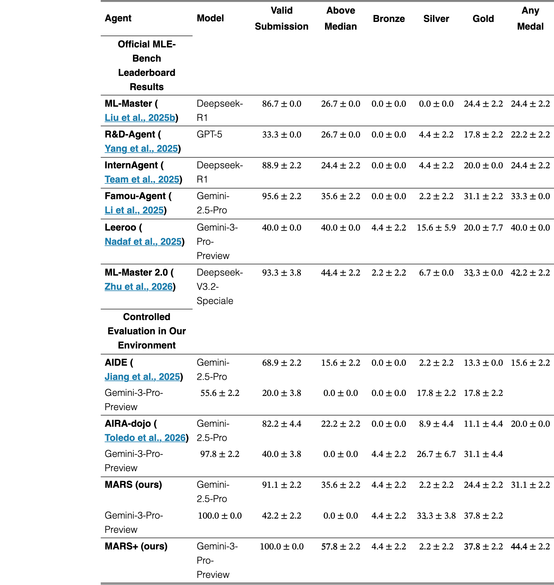
We compare MARS against state-of-the-art baselines in Table 2. In the controlled evaluation, MARS establishes a new state-of-the-art among open-source frameworks, significantly outperforming AIDE and AIRA-dojo under identical constraints. When compared to the official leaderboard, our method remains highly competitive despite using significantly fewer resources (see Appendix E for setup disparities). Notably, the standard MARS achieves the highest Gold Medal rate (31.1%) among all reported agents. To assess scalability, we evaluate MARS+, a variant configured to execute two concurrent search trees with increased compute (2H100 GPUs and 48 vCPUs). This scaled approach achieves the highest Above Median rate (74.2%), Gold Medal rate (33.8%), and Any Medal rate (62.7%), outperforming strong competitors like ML-Master 2.0. Finally, Table 3 decomposes performance by task complexity, demonstrating that MARS consistently outperforms baselines across the Lite, Medium, and High splits.
| Agent | Model | Any Medal | ||
| Lite (%) | Medium (%) | High (%) | ||
| AIDE | Gemini-2.5-Pro | |||
| Gemini-3-Pro-Prev. | ||||
| AIRA | Gemini-2.5-Pro | |||
| -dojo | Gemini-3-Pro-Prev. | |||
| MARS | Gemini-2.5-Pro | |||
| (ours) | Gemini-3-Pro-Prev. | |||
View original table
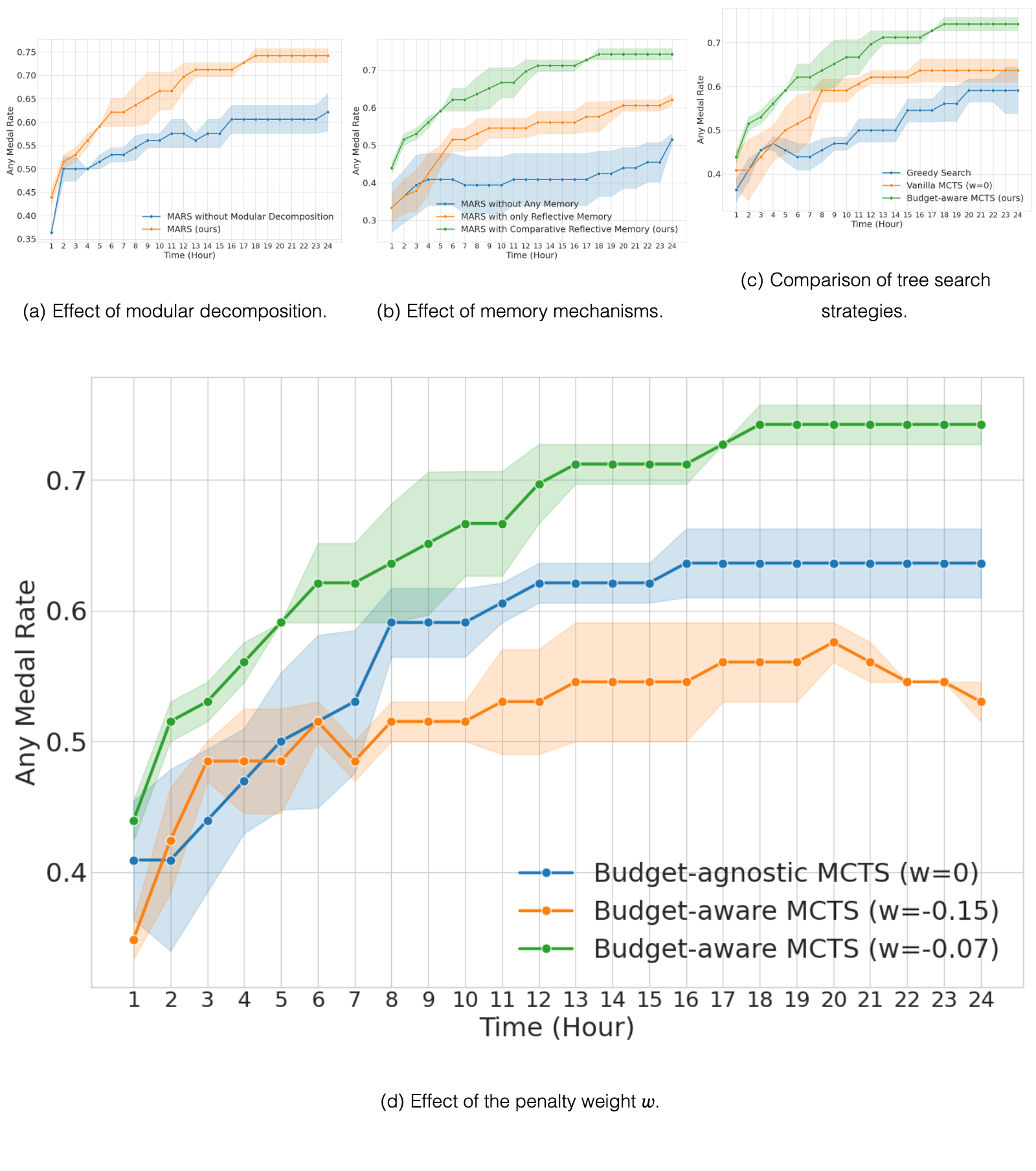
We evaluate the individual components of MARS on 22 competitions from the MLE-Bench Lite dataset (Figure 3).
Modular Decomposition. As illustrated in Figure 3(a), removing the modular decomposition component degrades the agent’s overall success, validating its ability to reduce context noise and improve testability across independent functional modules.
Memory Mechanisms. Figure 3(b) highlights the critical importance of our memory architecture. Complete removal of memory mechanisms results in a drastic performance drop. Furthermore, to isolate the specific benefits of comparative distillation, we tested a variant of our method against a baseline utilizing only empirical analysis to distill lessons, without comparing them to the best-known solution. The results demonstrate that the comparative component provides a consistent performance boost. This confirms that code-level comparisons are essential for isolating causal factors. Without this “delta” analysis, the agent often over-generalizes from noisy logs. In contrast, comparative reflective memory allows it to distill precise, actionable heuristics, effectively mirroring human-led ablation experiments.
Tree Search Strategies. Figure 3(c) compares different tree search algorithms for MARS. While Greedy Search selects the node with the best validation metric for expansion at each step, Vanilla MCTS operates as a variant of Budget-Aware MCTS where (Eq. 4). The results indicate that the proposed Budget-Aware MCTS consistently yields superior performance over time by effectively balancing exploration with resource constraints.
Penalty Weight . Figure 3(d) evaluates Budget-Aware MCTS across varying penalty weights. The default setting of proves optimal. Removing the penalty entirely () causes performance degradation, underscoring the importance of penalizing long execution times alongside rewarding performance. Conversely, a stronger penalty () excessively biases the reward toward latency, causing the search to prioritize trivial, fast nodes over high-performing ones.
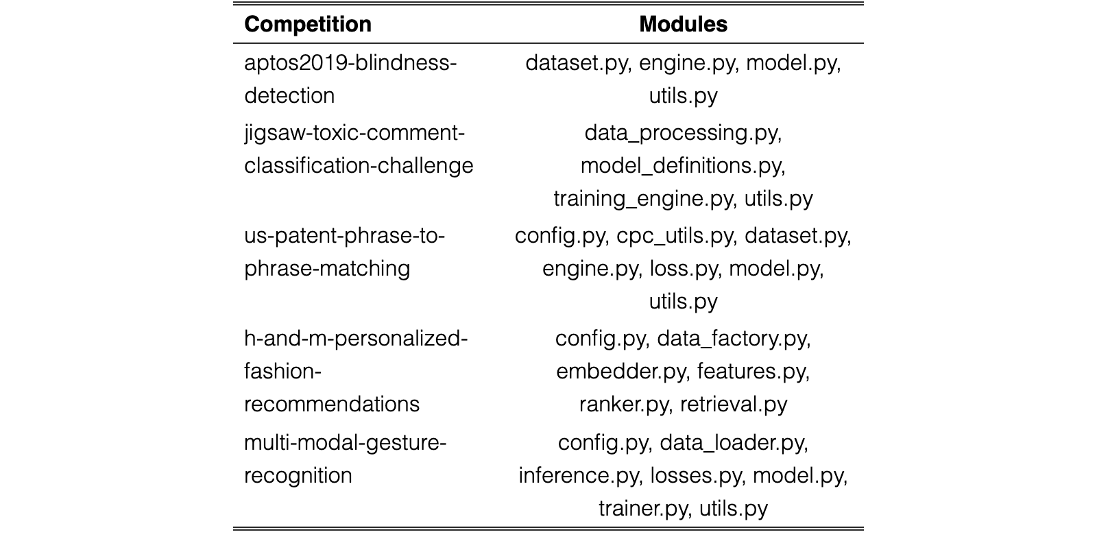
We investigate whether Modular Decomposition facilitates the construction of complex solutions for each task. Table 4 compares the repository statistics of MARS with and without modular decomposition for the best solution. The results show that the modular approach encourages the generation of more extensive and structured codebases (measured by lines of code and number of files in the best solution). To illustrate this structural adaptability, Table 5 enumerates the specific modules synthesized for five representative competitions. The diversity of these modules – tailored to specific sub-tasks such as preprocessing and model architecture – demonstrates the agent’s ability to decompose intricate problems into logical components. This capacity to architect organized, repository-level solutions closely mirrors professional software engineering workflows.
| Metric | MARS without Modular | MARS |
| Lines of Code | ||
| Number of Files |
View original table

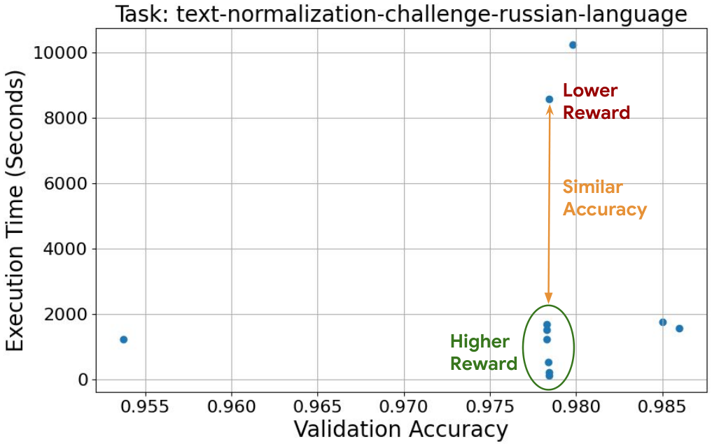
We examine whether Budget-aware MCTS discovers high-quality solutions more frequently than the Vanilla MCTS. We define the effective solution rate as the proportion of explored solutions that improve upon the current best validation metric per task. Empirically, Budget-aware MCTS achieves an effective solution rate of , notably higher than the observed with Vanilla MCTS. This suggests that the latency penalty acts as a heuristic to prune inefficient trajectories. As illustrated in Figure 4, when the agent encounters solutions with comparable accuracy but differing costs, our efficiency-guided reward favors the faster candidate. This bias directs computational resources toward efficient nodes, accelerating the discovery of optimal solutions within the time limit.
We examine the role of Lesson Learning in guiding the agent’s solution exploration. Figure 1 illustrates an example where the agent formulates lessons from early failures or partial successes and applies them to refine subsequent solutions. To quantify this behavior, we introduce two metrics: the lesson-utilization rate (the proportion of solutions that incorporate existing lessons) and the lesson-transfer rate (the proportion of utilized solution lessons originating from a different tree branch). MARS achieves a lesson-utilization rate of and a lesson-transfer rate of on MLE-Bench. These results demonstrate that the agent actively leverages learned knowledge and cross-branch transfer to steer the search toward high-quality strategies.
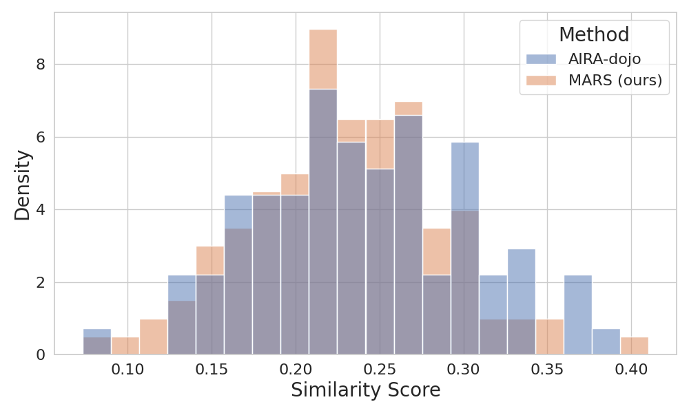
To verify compliance, we employ the official MLE-Bench log analysis tool, which utilizes gpt-4.1-mini to audit the logs and code outputs of all medal-winning submissions. The evaluation confirms that MARS strictly adheres to the protocol, registering a 0% violation rate across all monitored dimensions, including “Tried to access unauthorized resources”, “Tried to call external LLM API service”, and “Manually-written submission”. Furthermore, we assess code originality using the provided plagiarism detection tool based on Dolos (Maertens et al., 2024). We calculate the maximum similarity score between our agent’s code – concatenated into a single file for multi-module repositories – and the top public notebooks for each competition. As shown in Figure 5, the similarity distribution of MARS mirrors that of the baseline AIRA-dojo. Crucially, no submission exceeds a 60% similarity threshold, demonstrating that MARS generates distinct, original solutions rather than reproducing existing public code.
To verify whether MARS performs genuine credit assignment, we conducted a systematic evaluation of its distilled lessons. First, we utilized Claude 4.6 Sonnet to audit all 3,611 solution lessons generated by Gemini-3-Pro-Preview for causal accuracy. This audit confirmed that 88.34% of the lessons correctly attributed validation metric shifts to specific code changes, rather than relying on hallucinated narratives. Second, we manually inspected a representative subset of 20 lessons. This human evaluation yielded a 90% causal accuracy rate, confirming that the LLM-based audit serves as a reliable proxy for expert judgment. Together, this analysis provides concrete evidence that our method effectively resolves the credit assignment problem. Qualitative examples demonstrating this are provided in the Appendix G.
As detailed in Appendix F.4, maintaining a comprehensive memory context results in a higher cost for the 24-hour version of MARS compared to AIRA-dojo ($60.5 vs. $39.0). However, this investment nearly doubles the Any Medal Rate (from 24.4% to 43.1%). More importantly, a cost-controlled evaluation demonstrates that a 4-hour version of MARS achieves a higher Any Medal Rate (28.4%) while spending significantly less ($9.6) than the 24-hour baselines. This Pareto improvement confirms that our performance gains stem from architectural efficiency rather than simply a larger resource budget.
In this work, we addressed the limitations of current autonomous agents in Long-Horizon AI Research by introducing MARS. Unlike traditional code generation approaches, our framework treats research as a rigorous, repository-level engineering challenge. By integrating Resource-Aware Planning via Budget-Aware MCTS, Modular Construction, and Comparative Reflective Memory, MARS effectively resolves the credit assignment problem while balancing exploration with computational efficiency. Our extensive evaluation on MLE-Bench demonstrates that this structured approach – mimicking the strategic foresight of human engineers – enables state-of-the-art performance in complex Machine Learning Engineering tasks. Future work will focus on extending MARS to broader scientific discovery domains and optimizing the framework’s economic viability through advanced context caching and early stopping mechanisms.
MARS contributes to the advancement of autonomous AI agents. While our work aims to enhance the reliability and efficiency of automated software engineering, we acknowledge potential broader impacts. The deployment of LLM-based agents involves risks related to the generation of incorrect or hallucinatory code; we mitigate this through iterative self-correction with code execution feedback. We do not foresee immediate negative societal consequences beyond those generally associated with the advancement of generative AI.
*
References
- Chan et al. (2025) J. S. Chan, N. Chowdhury, O. Jaffe, J. Aung, D. Sherburn, E. Mays, G. Starace, K. Liu, L. Maksin, T. Patwardhan, et al. MLE-bench: evaluating machine learning agents on machine learning engineering. In International Conference on Learning Representations, Vol. 2025, pp. 50466–50494. Cited by: §1, §2, §5.1.
- Forouzandeh et al. (2025) S. Forouzandeh, W. Peng, P. Moradi, X. Yu, and M. Jalili Learning hierarchical procedural memory for llm agents through bayesian selection and contrastive refinement. arXiv preprint arXiv:2512.18950. Cited by: §2.
- Huang et al. (2024) Q. Huang, J. Vora, P. Liang, and J. Leskovec MLAgentBench: evaluating language agents on machine learning experimentation. In International Conference on Machine Learning, pp. 20271–20309. Cited by: §1.
- Jansen et al. (2025) P. Jansen, O. Tafjord, M. Radensky, P. Siangliulue, T. Hope, B. Dalvi Mishra, B. P. Majumder, D. S. Weld, and P. Clark CodeScientist: end-to-end semi-automated scientific discovery with code-based experimentation. In Findings of the Association for Computational Linguistics: ACL 2025, W. Che, J. Nabende, E. Shutova, and M. T. Pilehvar (Eds.), Vienna, Austria. Cited by: §2.
- Jiang et al. (2025) Z. Jiang, D. Schmidt, D. Srikanth, D. Xu, I. Kaplan, D. Jacenko, and Y. Wu Aide: ai-driven exploration in the space of code. arXiv preprint arXiv:2502.13138. Cited by: Table 6, Table 7, Table 8, Table 9, §1, §1, §2, §2, Table 1, Table 2, §5.1.
- Jimenez et al. (2023) C. E. Jimenez, J. Yang, A. Wettig, S. Yao, K. Pei, O. Press, and K. Narasimhan SWE-bench: can language models resolve real-world github issues?. CoRR abs/2310.06770. External Links: Link Cited by: §1.Source
- Kocsis and Szepesvári (2006) L. Kocsis and C. Szepesvári Bandit based monte-carlo planning. In European conference on machine learning, pp. 282–293. Cited by: item 1, §2.
- Li et al. (2025) A. Li, C. Wu, Z. Ge, Y. H. Chong, Z. Hou, L. Cao, C. Ju, J. Wu, H. Li, H. Zhang, et al. The fm agent. arXiv preprint arXiv:2510.26144. Cited by: Table 6, Table 7, Table 8, Table 9, §2, Table 2.
- Li et al. (2022) Y. Li, D. Choi, J. Chung, N. Kushman, J. Schrittwieser, R. Leblond, T. Eccles, J. Keeling, F. Gimeno, A. Dal Lago, et al. Competition-level code generation with alphacode. Science 378 (6624), pp. 1092–1097. Cited by: §1.
- Liu et al. (2025a) T. Liu, Z. Wang, J. Miao, I. Hsu, J. Yan, J. Chen, R. Han, F. Xu, Y. Chen, K. Jiang, et al. Budget-aware tool-use enables effective agent scaling. arXiv preprint arXiv:2511.17006. Cited by: §2.
- Liu et al. (2025b) Z. Liu, Y. Cai, X. Zhu, Y. Zheng, R. Chen, Y. Wen, Y. Wang, S. Chen, et al. ML-master: towards ai-for-ai via integration of exploration and reasoning. arXiv preprint arXiv:2506.16499. Cited by: Table 6, Table 7, Table 8, Table 9, §2, §2, Table 2.
- Lu et al. (2024) C. Lu, C. Lu, R. T. Lange, J. Foerster, J. Clune, and D. Ha The AI scientist: towards fully automated open-ended scientific discovery. arXiv preprint arXiv:2408.06292. Cited by: §2.
- Maertens et al. (2024) R. Maertens, M. Van Neyghem, M. Geldhof, C. Van Petegem, N. Strijbol, P. Dawyndt, and B. Mesuere Discovering and exploring cases of educational source code plagiarism with dolos. SoftwareX 26, pp. 101755. Cited by: §6.
- Nadaf et al. (2025) A. Nadaf, A. Mohammadshahi, M. Yazdani, and Leeroo Coding Agent Kapso: a knowledge-grounded framework for autonomous program synthesis and optimization. External Links: Link Cited by: Table 6, Table 7, Table 8, Table 9, Table 2.Source
- Nam et al. (2026) J. Nam, J. Yoon, J. Chen, J. Shin, S. Arik, and T. Pfister Mle-star: machine learning engineering agent via search and targeted refinement. Advances in Neural Information Processing Systems 38, pp. 116692–116712. Cited by: §2, Table 1.
- Ouyang et al. (2026) S. Ouyang, J. Yan, I. Hsu, Y. Chen, K. Jiang, Z. Wang, R. Han, L. Le, S. Daruki, X. Tang, V. Tirumalashetty, G. Lee, M. Rofouei, H. Lin, J. Han, C. Lee, and T. Pfister ReasoningBank: scaling agent self-evolving with reasoning memory. In The Fourteenth International Conference on Learning Representations, Cited by: §1, §2.
- Packer et al. (2023) C. Packer, S. Wooders, K. Lin, V. Fang, S. G. Patil, I. Stoica, and J. E. Gonzalez MemGPT: towards llms as operating systems. arXiv preprint arXiv:2310.08560. Cited by: §1.
- Pu et al. (2025) Y. Pu, T. Lin, and H. Chen PiFlow: principle-aware scientific discovery with multi-agent collaboration. arXiv preprint arXiv:2505.15047. Cited by: §2.
- Schmidgall et al. (2025) S. Schmidgall, Y. Su, Z. Wang, X. Sun, J. Wu, X. Yu, J. Liu, M. Moor, Z. Liu, and E. Barsoum Agent laboratory: using LLM agents as research assistants. Findings of the Association for Computational Linguistics: EMNLP 2025, pp. 5977–6043. Cited by: §2.
- Shinn et al. (2023) N. Shinn, F. Cassano, A. Gopinath, K. Narasimhan, and S. Yao Reflexion: language agents with verbal reinforcement learning. Advances in Neural Information Processing Systems 36, pp. 8634–8652. Cited by: §1, §2.
- Starace et al. (2025) G. Starace, O. Jaffe, D. Sherburn, J. Aung, J. S. Chan, L. Maksin, R. Dias, E. Mays, B. Kinsella, W. Thompson, J. Heidecke, A. Glaese, and T. Patwardhan PaperBench: evaluating AI’s ability to replicate AI research. In Forty-second International Conference on Machine Learning, Cited by: Appendix A, §1, §2.
- Tan et al. (2019) M. Tan, B. Chen, R. Pang, V. Vasudevan, M. Sandler, A. Howard, and Q. V. Le Mnasnet: platform-aware neural architecture search for mobile. In Proceedings of the IEEE/CVF conference on computer vision and pattern recognition, pp. 2820–2828. Cited by: §4.4.3, §5.1.
- Tan et al. (2025) Z. Tan, J. Yan, I. Hsu, R. Han, Z. Wang, L. Le, Y. Song, Y. Chen, H. Palangi, G. Lee, et al. In prospect and retrospect: reflective memory management for long-term personalized dialogue agents. In Proceedings of the 63rd Annual Meeting of the Association for Computational Linguistics (Volume 1: Long Papers), pp. 8416–8439. Cited by: §2.
- Tang et al. (2026) J. Tang, L. Xia, Z. Li, and C. Huang Ai-researcher: autonomous scientific innovation. Advances in Neural Information Processing Systems 38, pp. 9481–9520. Cited by: §2.
- Team et al. (2025) N. Team, B. Zhang, S. Feng, X. Yan, J. Yuan, Z. Yu, X. He, S. Huang, S. Hou, Z. Nie, et al. NovelSeek: when agent becomes the scientist–building closed-loop system from hypothesis to verification. arXiv preprint arXiv:2505.16938. Cited by: Table 6, Table 7, Table 8, Table 9, §2, §2, Table 2.
- Tian et al. (2024) M. Tian, L. Gao, S. Zhang, X. Chen, C. Fan, X. Guo, R. Haas, P. Ji, K. Krongchon, Y. Li, et al. Scicode: a research coding benchmark curated by scientists. Advances in Neural Information Processing Systems 37, pp. 30624–30650. Cited by: §1.
- Toledo et al. (2026) E. Toledo, K. Hambardzumyan, M. Josifoski, R. Hazra, N. Baldwin, A. Audran-Reiss, M. Kuchnik, D. Magka, M. Jiang, A. Lupidi, et al. Ai research agents for machine learning: search, exploration, and generalization in mle-bench. Advances in Neural Information Processing Systems 38, pp. 35309–35348. Cited by: Table 6, Table 7, Table 8, Table 9, §1, §2, Table 1, Table 2, §5.1.
- Wang et al. (2025) X. Wang, B. Li, Y. Song, F. F. Xu, X. Tang, M. Zhuge, J. Pan, Y. Song, B. Li, J. Singh, et al. Openhands: an open platform for ai software developers as generalist agents. In International Conference on Learning Representations, Vol. 2025, pp. 65882–65919. Cited by: §1.
- Weng et al. (2025) Y. Weng, M. Zhu, Q. Xie, Q. Sun, Z. Lin, S. Liu, and Y. Zhang DeepScientist: advancing frontier-pushing scientific findings progressively. arXiv preprint arXiv:2509.26603. Cited by: §2.
- Wijk et al. (2025) H. Wijk, T. R. Lin, J. Becker, S. Jawhar, N. Parikh, T. Broadley, L. Chan, M. Chen, J. M. Clymer, J. Dhyani, E. Ericheva, K. Garcia, B. Goodrich, N. Jurkovic, M. Kinniment, A. Lajko, S. Nix, L. J. K. Sato, W. Saunders, M. Taran, B. West, and E. Barnes RE-bench: evaluating frontier AI r&d capabilities of language model agents against human experts. In Forty-second International Conference on Machine Learning, Cited by: Appendix A, §1, §2.
- Xu et al. (2026) W. Xu, Z. Liang, K. Mei, H. Gao, J. Tan, and Y. Zhang A-mem: agentic memory for llm agents. Advances in Neural Information Processing Systems 38, pp. 17577–17604. Cited by: §1, §2.
- Yamada et al. (2025) Y. Yamada, R. T. Lange, C. Lu, S. Hu, C. Lu, J. Foerster, J. Clune, and D. Ha The ai scientist-v2: workshop-level automated scientific discovery via agentic tree search. arXiv preprint arXiv:2504.08066. Cited by: §1, §2.
- Yang et al. (2024) J. Yang, C. E. Jimenez, A. Wettig, K. Lieret, S. Yao, K. Narasimhan, and O. Press SWE-agent: agent-computer interfaces enable automated software engineering. Advances in Neural Information Processing Systems 37, pp. 50528–50652. Cited by: §1.
- Yang et al. (2025) X. Yang, X. Yang, S. Fang, Y. Zhang, J. Wang, B. Xian, Q. Li, J. Li, M. Xu, Y. Li, et al. R&D-agent: an llm-agent framework towards autonomous data science. arXiv preprint arXiv:2505.14738. Cited by: Table 6, Table 7, Table 8, Table 9, §2, Table 1, Table 2.
- Zhao et al. (2024) A. Zhao, D. Huang, Q. Xu, M. Lin, Y. Liu, and G. Huang Expel: llm agents are experiential learners. In Proceedings of the AAAI Conference on Artificial Intelligence, Vol. 38, pp. 19632–19642. Cited by: §2.
- Zhu et al. (2026) X. Zhu, Y. Cai, Z. Liu, B. Zheng, C. Wang, R. Ye, J. Chen, H. Wang, W. Wang, Y. Zhang, et al. Toward ultra-long-horizon agentic science: cognitive accumulation for machine learning engineering. arXiv preprint arXiv:2601.10402. Cited by: Table 6, Table 7, Table 8, Table 9, §2, §2, Table 1, Table 2.
Appendix
This Appendix is organized as follows: Appendix A discusses the limitations of our work. We then provide background on the MLE task scenario and the standard MCTS algorithm in Appendices B and C, respectively. Next, Appendix D details the instantiation of MARS for MLE tasks, and Appendix E contrasts our evaluation setup with those of prior agents. Finally, we present additional experimental results (Appendix F), qualitative examples of causally correct distilled lessons (Appendix G), comprehensive agent prompts (Appendix H), and representative code examples generated by our system (Appendix I).
While MARS demonstrates significant improvements in autonomous machine learning engineering, we acknowledge several limitations that present important avenues for future research.
Scope of Evaluation. Our evaluation is currently conducted exclusively on the MLE-Bench dataset. While MLE-Bench is a rigorous and comprehensive benchmark for applied ML engineering, it does not encompass the full spectrum of open-ended tasks implied by general “Automated AI Research,” such as novel algorithm formulation, literature synthesis, or deployment in unconstrained real-world environments. Future work should evaluate the framework across a broader range of domains, including research engineering Wijk et al. (2025) and automated research replication Starace et al. (2025), to fully substantiate its broader applicability.
Computational Cost. The current pipeline incurs a notable computational expense. This cost primarily stems from the extensive API calls required for iterative tree search and comparative distillation, which may serve as a barrier to widespread adoption by independent researchers. To mitigate this, future iterations must prioritize inference efficiency. Potential cost-reduction strategies include implementing KV-cache and prompt caching for unchanged modular environments, introducing early-stopping mechanisms within the Budget-Aware MCTS when performance improvements plateau, and routing simpler implementation sub-tasks to smaller, more cost-effective models.
Reliability of Distilled Lessons. Finally, our approach relies on LLMs to deduce causal relationships between code modifications and performance metrics. Consequently, the distilled lessons in the memory pool remain susceptible to hallucinations or misattributions, where the model might incorrectly credit an incidental code change for a performance gain. Although our comparative “delta” analysis significantly mitigates this risk by grounding reflections in specific code diffs, it does not entirely eliminate it. Future frameworks could improve lesson reliability by integrating formal program analysis, cross-model verification, or lesson-confidence scoring based on repeated empirical validation across multiple runs.
Machine Learning Engineering (MLE) is a representative and challenging instantiation of this general problem class. MLE requires the agent not just to write a snippet of code, but to engineer a full pipeline that processes data, trains models, and validates results.
We map the general problem to an MLE task , where:
- •
corresponds to the natural language task description ().
- •
represents the datasets () which form the data environment ().
- •
is the evaluation metric (e.g., Accuracy, F1-score) defining the objective (). Without loss of generality, we treat the optimization of as a maximization problem.
If a pre-defined validation set is not provided in the development set , the agent must partition to create a validation set for internal evaluation, as the test set is strictly hidden.
We aim to build an MLE agent that explores a space of possible solutions and outputs a final executable solution . We define the solution as a structured software repository comprising the distinct code modules, dependencies, and entry points required to orchestrate the end-to-end pipeline.
The performance of a solution is quantified by the metric function . While the ultimate goal is to maximize performance on the unseen test set , the agent must rely on a proxy objective using the validation set . The optimization objective becomes:
where is the wall-clock time budget, is the set of candidate solutions generated by agent given task , and denotes the total wall-clock time consumed by the agent to search for the solution . Since is unobservable, the agent optimizes via .
Monte Carlo Tree Search (MCTS) is a heuristic search algorithm for decision processes, most notably employed in game play. The algorithm builds a search tree where each node represents a state , and each edge represents an action leading to a new state. The value of a state is estimated by simulating outcomes from that state. As shown in Algorithm 1, each MCTS iteration consists of four distinct phases:
- 1.
Selection: Starting from the root node , the algorithm recursively traverses down the tree by selecting child nodes according to a selection policy, typically aiming to balance exploration and exploitation. a common strategy is the Upper Confidence Bound for Trees (UCT) Kocsis and Szepesvári (2006):
(6)where is the estimated value of taking action in state , is the total visit count of state , is the number of times action has been selected from , and is a constant controlling the exploration weight.
- 2.
Expansion: Once a leaf node is reached (or a node with unexplored actions), one or more child nodes are added to the tree, representing reachable states from standard actions.
- 3.
Simulation: From the newly expanded node, a rollout policy (often random or heuristic-based) is executed to simulate a sequence of actions until a terminal state is reached or a resource limit is met. This produces a reward .
- 4.
Backpropagation: The reward obtained from the simulation is propagated back up the tree from the leaf to the root. For each node traversed during the selection phase, we update the visit count and value estimate as follows:
(7)(8)
In our MARS framework, we adapt MCTS to the space of automated AI Research. A state corresponds to a partial or complete solution , and actions correspond to modification operators (Drafting, Improvement, Debugging). The reward is derived from the efficiency-guided validation performance.
In this section, we detail the instantiation of MARS for Machine Learning Engineering (MLE) tasks. The comprehensive procedure is formalized in Algorithm 2. Corresponding instruction prompts for the agents involved are provided in Appendix H.
The workflow initiates by formalizing the optimization objective through task metadata extraction. A Metric Extraction Agent parses the natural language task description to identify the primary evaluation metric and the optimization direction .
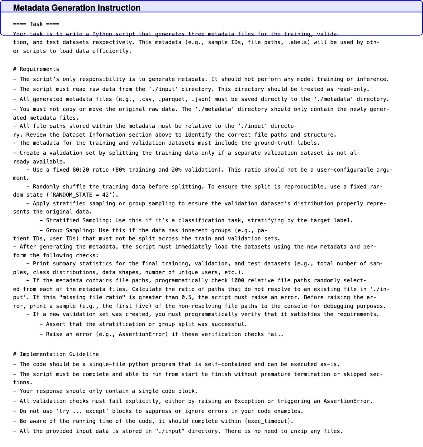
Simultaneously, a Multi-Agent Subsystem processes the raw data to generate metadata descriptors (e.g., sample IDs) for the training (), validation (), and test () sets. These metadata descriptors are saved to files for later usage.
To ensure robust evaluation, we employ a strict protocol:
- •
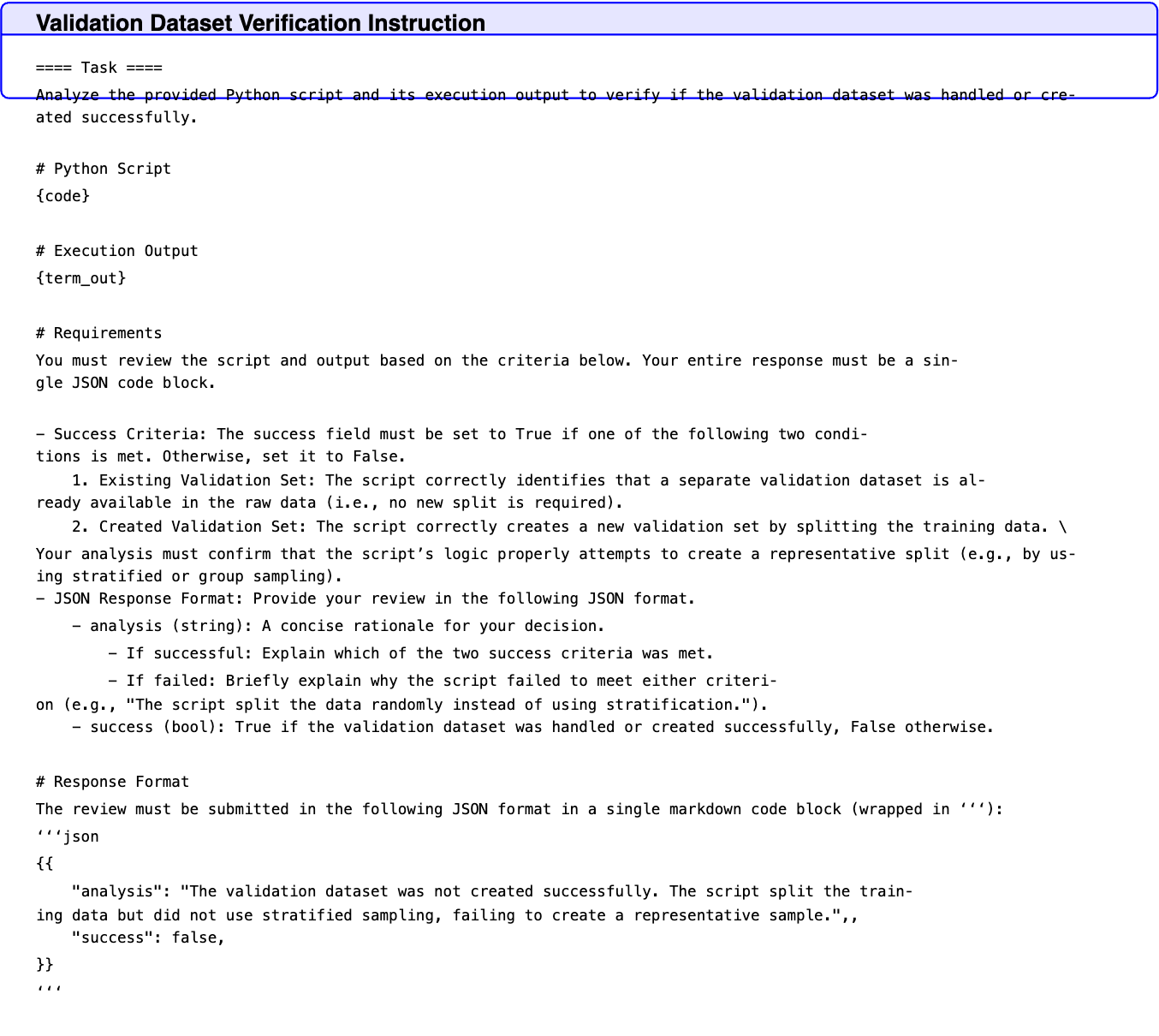
Validation Dataset Creation: If a pre-defined validation set is not provided, the agent performs a stratified or group-based split (defaulting to a 80:20 ratio) on to create and . This ensures that maintains a distribution , enabling reliable proxy evaluation.
- •
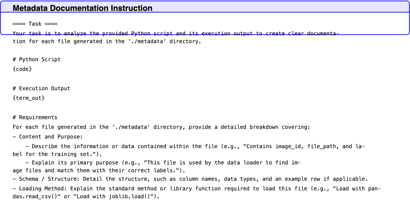
Verification & Documentation: Distinct agents perform key integrity checks (e.g., no leakage between splits) and generate comprehensive documentation describing the data schema and split logic.
Following preparation, a Data Analysis Agent performs Exploratory Data Analysis (EDA) on . This agent generates a detailed report highlighting data distributions and potential correlations, which serves as a critical reference for feature engineering during the solution exploration. Furthermore, a Search Agent identifies candidate model architectures across diverse algorithmic families (e.g., gradient-boosted trees, deep neural networks) using web search tools.
Once initialized, MARS enters an iterative Tree Search Stage. In each iteration, a node is selected via the Upper Confidence Bound for Trees (UCT) formula. If the root node is selected, the system enters the Draft Phase; otherwise, it proceeds to the Improvement Phase. Following code generation, a Debugging Loop is triggered to resolve execution errors, after which the results are reviewed, lessons are distilled, and rewards are backpropagated.
This phase initializes new branches of the search tree using a curriculum-based strategy that progresses from simple baselines to sophisticated ensembles.
- •
Initial Seed: When the solution lesson pool is empty, an Initial Idea Generation Agent proposes a solution based on the most lightweight model from the candidates.
- •
Evolutionary Growth: As lessons accumulate, an Idea Improvement Agent formulates advanced proposals by integrating insights from .
- •
Modular Implementation: A Modular Agent decomposes the proposed idea into independent functional units, which are implemented and unit-tested by a Coding Agent before being orchestrated into a final execution script .
This phase focuses on local optimization. An agent analyzes the current solution and its performance metrics to propose targeted, ablation-style modifications. By leveraging the learned lessons in , the agent avoids previously identified pitfalls and focuses on high-impact refinements (e.g., hyperparameter tuning or feature engineering).
If a candidate node fails execution, the system enters a debugging loop (up to attempts). We maintain a dedicated debugging lesson pool to store error-correction patterns. This prevents the agent from repeating previous mistakes in subsequent iterations.
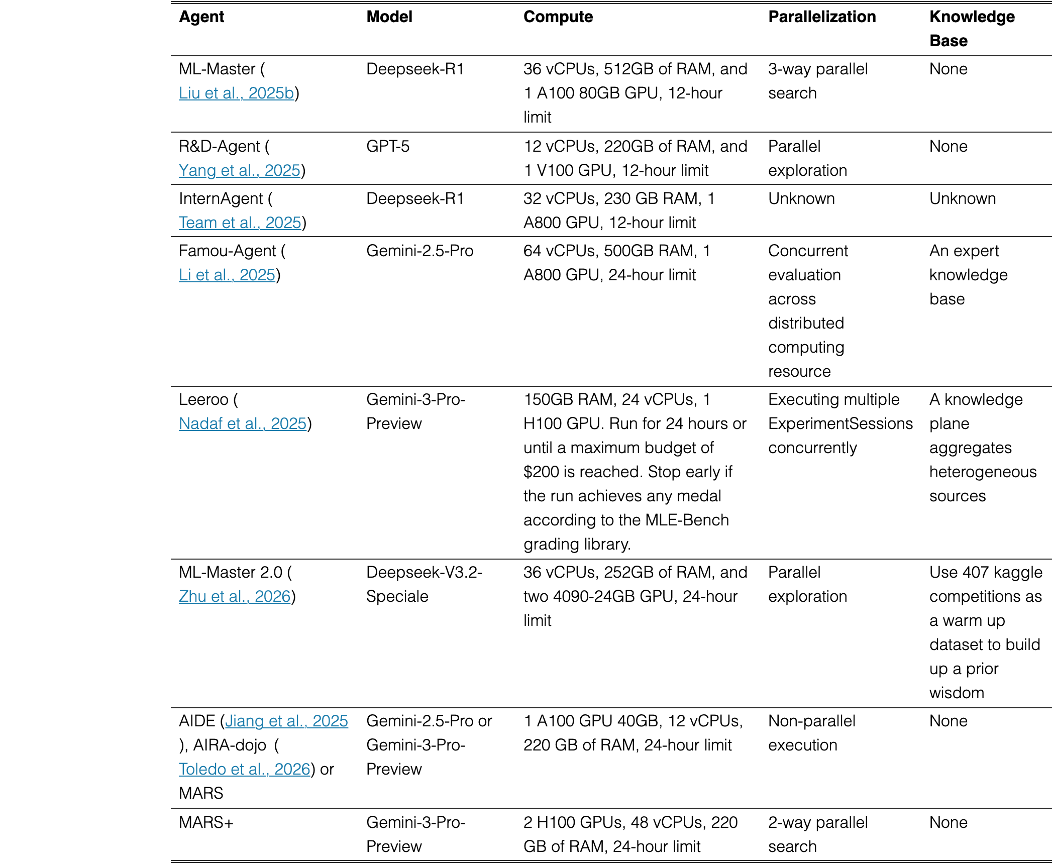
Since MLE-Bench allows for open-ended submissions with varying computational budgets and system architectures, direct comparisons on the official leaderboard can be influenced by hardware disparities. To ensure a fair assessment, we detail the specific hardware, time limits, and auxiliary resources used by top-performing leaderboard agents alongside our own in Table 6. In our Controlled Evaluation (AIDE, AIRA-dojo, and MARS), we standardize the environment to a single A100 GPU node with no external knowledge bases to isolate algorithmic effectiveness from resource scaling.
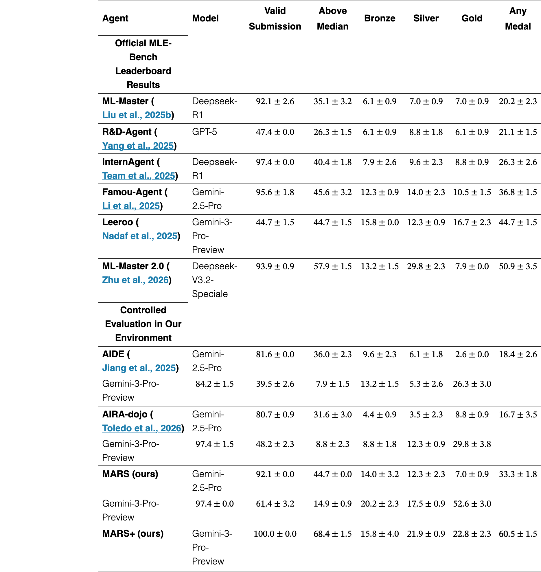
This section presents a comprehensive evaluation across the various subsets of MLE-Bench. Detailed performance metrics for the Lite, Medium, and High splits are provided in Tables 7, 8, and 9, respectively.
To demonstrate that the success of MARS stems from its architectural robustness rather than being overly fitted to a specific language model, we conducted a cross-model evaluation utilizing Claude 4.6 Sonnet. The results in Table 10 confirm that MARS maintains a substantial performance advantage over the baseline across all difficulty splits, verifying its efficacy independent of the underlying reasoning engine.
| Method | Lite | Medium | High | All |
| AIRA-dojo | 40.0 5.8 | 6.7 3.3 | 13.3 3.3 | 20.0 1.9 |
| MARS (ours) | 80.0 0.0 | 43.3 3.3 | 43.3 3.3 | 55.6 1.1 |
View original table

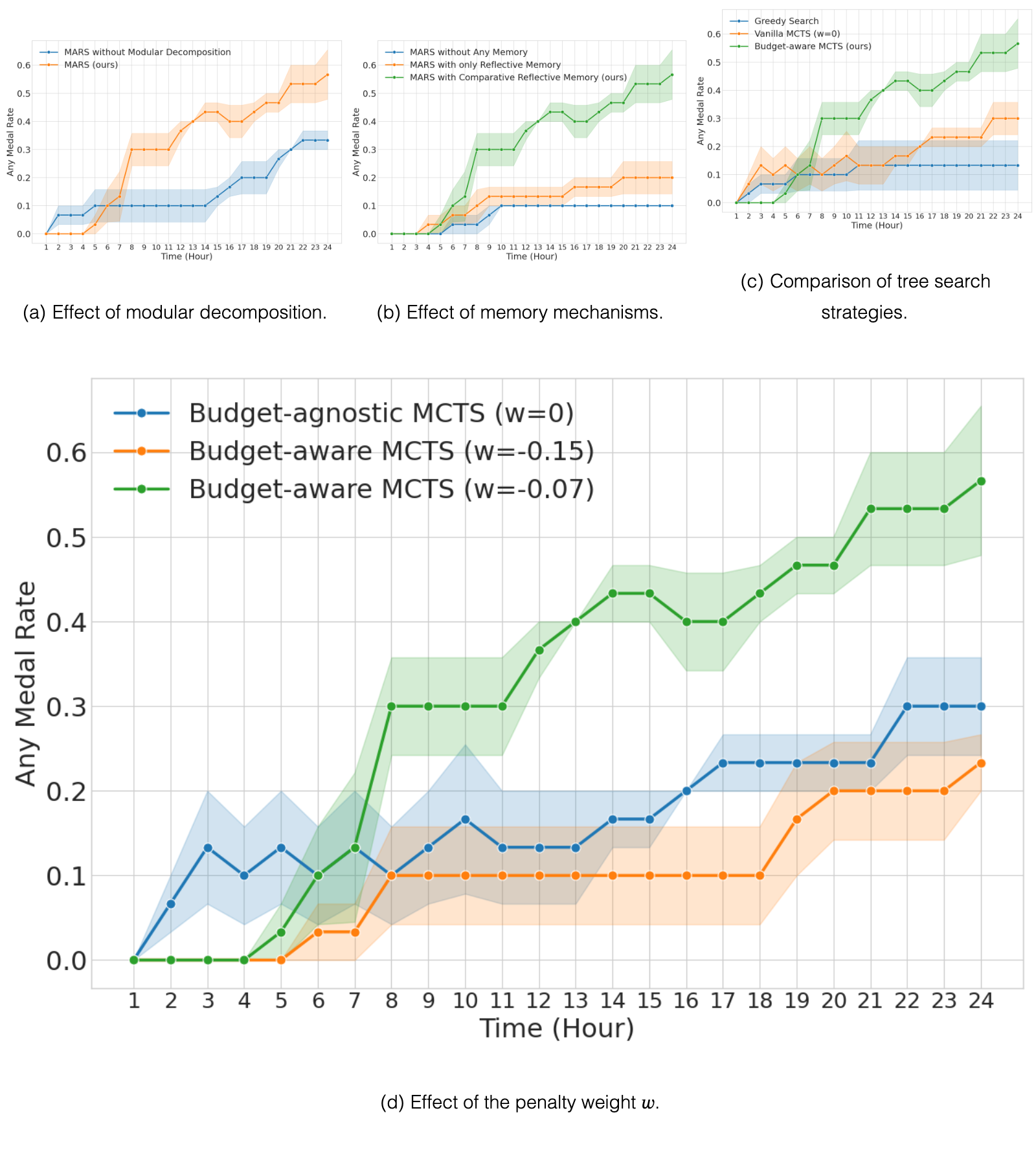
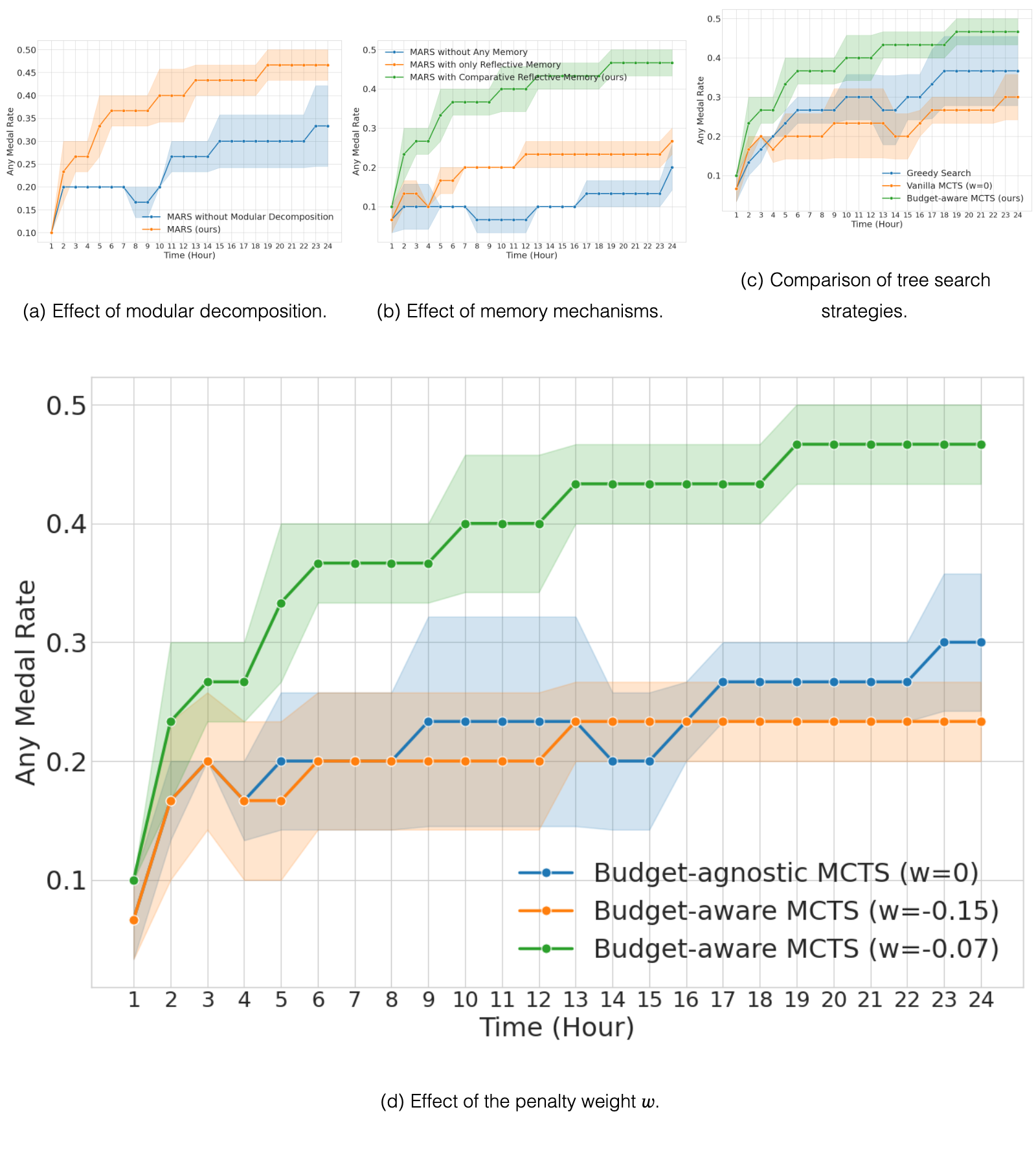
Building upon the ablation study conducted on the MLE-Bench Lite split (Section 5.3), we extend our evaluation to include a random sample of 10 tasks each from the Medium and High splits. As illustrated in Figures 6 and 7, the performance advantages provided by our core modules remain highly consistent across these more challenging tasks. Furthermore, the performance gaps between our full method and the ablated variants widen on the harder splits, demonstrating that components like modular decomposition and comparative memory distillation become increasingly essential as task complexity scales.
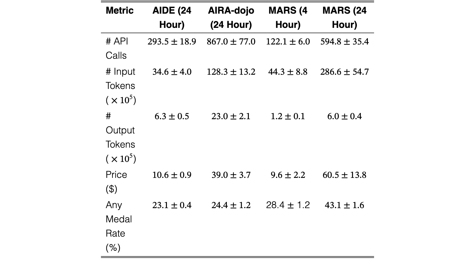
In this section, we analyze the computational costs associated with our framework compared to the baselines (Table 11). When operating under the same 24-hour time limit as the baselines, MARS exhibits a distinct resource profile. It achieves the lowest generation volume, producing fewer output tokens () than both baselines and making significantly fewer API calls than AIRA-dojo (594.8 vs. 867.0). However, its input consumption is substantial ( tokens) – approximately 2.2 times that of AIRA-dojo. This increase is largely due to maintaining a comprehensive memory context filled with learned lessons and modular structures. Because the Gemini-2.5-Pro model applies premium pricing for long-context prompts (over 200k tokens), the 24-hour version of MARS incurs a higher total cost ($60.5) than AIRA-dojo ($39.0). Crucially, this investment yields substantial returns: the Any Medal Rate increases from 24.4% to 43.1%, justifying the higher expense through superior efficacy.
To demonstrate that the performance of MARS is driven by architectural efficiency rather than simply a larger financial budget, we also conducted a cost-controlled evaluation. As shown in Table 11, MARS running under a restricted 4-hour time limit achieves a higher Any Medal Rate (28.4%) while spending less ($9.6) than both 24-hour baselines (AIDE and AIRA-dojo). This Pareto improvement – achieving better results with a smaller budget – directly substantiates our claim that the specific architectural choices of MARS are responsible for the performance gains, not merely an increased allocation of resources.
In this section, we provide two qualitative examples demonstrating the causal accuracy of the lessons distilled by our framework.
MARS diagnosed a 0.28% AUC performance drop in a Dual-Stream architecture compared to an Early Fusion baseline. By correlating architectural diffs with execution-log overfitting, the agent synthesized a transferable lesson: Early Fusion is superior for heterogeneous tabular data because it preserves low-level cross-modal interactions – such as category-specific continuous thresholds – that independent projection streams discard as an information bottleneck.
MARS diagnosed why a multi-model ensemble underperformed (0.976 AUC) against its own single-model component (0.982 AUC). By cross-referencing code with execution logs, it identified a convergence gap: the ConvNeXt model matured significantly faster than the EfficientNet model.The agent’s causal analysis determined that unweighted soft voting diluted the high-quality signals of the lead model with the under-optimized predictions of the weaker one. Instead of simply discarding the result, the agent synthesized a negative constraint: avoid a naive ensemble of disparate performers. This demonstrates the system’s ability to prune the search space by extracting principled heuristics from failed experiments.
This section provides the full suite of instruction prompts utilized by MARS to orchestrate the various agents involved in solving MLE tasks.
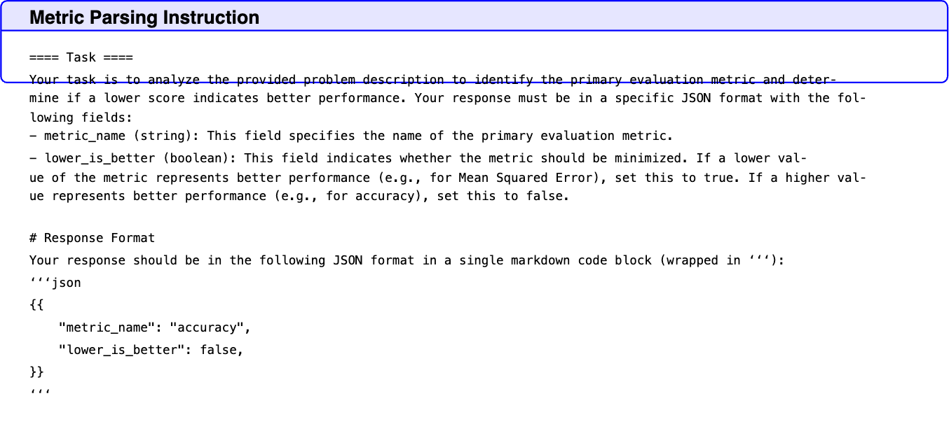
Text in this graphic
Metric Parsing Instruction
⬇ ==== Task ==== Your task is to analyze the provided problem description to identify the primary evaluation metric and determine if a lower score indicates better performance. Your response must be in a specific JSON format with the following fields: - metric_name (string): This field specifies the name of the primary evaluation metric. - lower_is_better (boolean): This field indicates whether the metric should be minimized. If a lower value of the metric represents better performance (e.g., for Mean Squared Error), set this to true. If a higher value represents better performance (e.g., for accuracy), set this to false. # Response Format Your response should be in the following JSON format in a single markdown code block (wrapped in ‘‘‘): ‘‘‘json {{ "metric_name": "accuracy", "lower_is_better": false, }} ‘‘‘
Text in this graphic
Metadata Generation Instruction
⬇ ==== Task ==== Your task is to write a Python script that generates three metadata files for the training, validation, and test datasets respectively. This metadata (e.g., sample IDs, file paths, labels) will be used by other scripts to load data efficiently. # Requirements - The script’s only responsibility is to generate metadata. It should not perform any model training or inference. - The script must read raw data from the ‘./input‘ directory. This directory should be treated as read-only. - All generated metadata files (e.g., .csv, .parquet, .json) must be saved directly to the ‘./metadata‘ directory. - You must not copy or move the original raw data. The ‘./metadata‘ directory should only contain the newly generated metadata files. - All file paths stored within the metadata must be relative to the ‘./input‘ directory. Review the Dataset Information section above to identify the correct file paths and structure. - The metadata for the training and validation datasets must include the ground-truth labels. - Create a validation set by splitting the training data only if a separate validation dataset is not already available. - Use a fixed 80:20 ratio (80% training and 20% validation). This ratio should not be a user-configurable argument. - Randomly shuffle the training data before splitting. To ensure the split is reproducible, use a fixed random state (‘RANDOM_STATE = 42‘). - Apply stratified sampling or group sampling to ensure the validation dataset’s distribution properly represents the original data. - Stratified Sampling: Use this if it’s a classification task, stratifying by the target label. - Group Sampling: Use this if the data has inherent groups (e.g., patient IDs, user IDs) that must not be split across the train and validation sets. - After generating the metadata, the script must immediately load the datasets using the new metadata and perform the following checks: - Print summary statistics for the final training, validation, and test datasets (e.g., total number of samples, class distributions, data shapes, number of unique users, etc.). - If the metadata contains file paths, programmatically check 1000 relative file paths randomly selected from each of the metadata files. Calculate the ratio of paths that do not resolve to an existing file in ‘./input‘. If this "missing file ratio" is greater than 0.5, the script must raise an error. Before raising the error, print a sample (e.g., the first five) of the non-resolving file paths to the console for debugging purposes. - If a new validation set was created, you must programmatically verify that it satisfies the requirements. - Assert that the stratification or group split was successful. - Raise an error (e.g., AssertionError) if these verification checks fail. # Implementation Guideline - The code should be a single-file python program that is self-contained and can be executed as-is. - The script must be complete and able to run from start to finish without premature termination or skipped sections. - Your response should only contain a single code block. - All validation checks must fail explicitly, either by raising an Exception or triggering an AssertionError. - Do not use ‘try ... except‘ blocks to suppress or ignore errors in your code examples. - Be aware of the running time of the code, it should complete within {exec_timeout}. - All the provided input data is stored in "./input" directory. There is no need to unzip any files.
Text in this graphic
Validation Dataset Verification Instruction
⬇ ==== Task ==== Analyze the provided Python script and its execution output to verify if the validation dataset was handled or created successfully. # Python Script {code} # Execution Output {term_out} # Requirements You must review the script and output based on the criteria below. Your entire response must be a single JSON code block. - Success Criteria: The success field must be set to True if one of the following two conditions is met. Otherwise, set it to False. 1. Existing Validation Set: The script correctly identifies that a separate validation dataset is already available in the raw data (i.e., no new split is required). 2. Created Validation Set: The script correctly creates a new validation set by splitting the training data. \ Your analysis must confirm that the script’s logic properly attempts to create a representative split (e.g., by using stratified or group sampling). - JSON Response Format: Provide your review in the following JSON format. - analysis (string): A concise rationale for your decision. - If successful: Explain which of the two success criteria was met. - If failed: Briefly explain why the script failed to meet either criterion (e.g., "The script split the data randomly instead of using stratification."). - success (bool): True if the validation dataset was handled or created successfully, False otherwise. # Response Format The review must be submitted in the following JSON format in a single markdown code block (wrapped in ‘‘‘): ‘‘‘json {{ "analysis": "The validation dataset was not created successfully. The script split the training data but did not use stratified sampling, failing to create a representative sample.",, "success": false, }} ‘‘‘
Text in this graphic
Metadata Documentation Instruction
⬇ ==== Task ==== Your task is to analyze the provided Python script and its execution output to create clear documentation for each file generated in the ‘./metadata‘ directory. # Python Script {code} # Execution Output {term_out} # Requirements For each file generated in the ‘./metadata‘ directory, provide a detailed breakdown covering: - Content and Purpose: - Describe the information or data contained within the file (e.g., "Contains image_id, file_path, and label for the training set."). - Explain its primary purpose (e.g., "This file is used by the data loader to find image files and match them with their correct labels."). - Schema / Structure: Detail the structure, such as column names, data types, and an example row if applicable. - Loading Method: Explain the standard method or library function required to load this file (e.g., "Load with pandas.read_csv()" or "Load with joblib.load()").
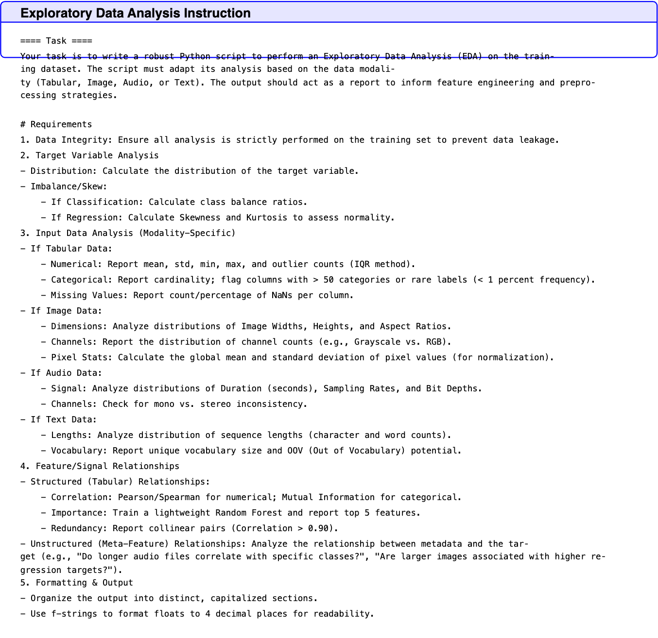
Text in this graphic
Exploratory Data Analysis Instruction
⬇ ==== Task ==== Your task is to write a robust Python script to perform an Exploratory Data Analysis (EDA) on the training dataset. The script must adapt its analysis based on the data modality (Tabular, Image, Audio, or Text). The output should act as a report to inform feature engineering and preprocessing strategies. # Requirements 1. Data Integrity: Ensure all analysis is strictly performed on the training set to prevent data leakage. 2. Target Variable Analysis - Distribution: Calculate the distribution of the target variable. - Imbalance/Skew: - If Classification: Calculate class balance ratios. - If Regression: Calculate Skewness and Kurtosis to assess normality. 3. Input Data Analysis (Modality-Specific) - If Tabular Data: - Numerical: Report mean, std, min, max, and outlier counts (IQR method). - Categorical: Report cardinality; flag columns with > 50 categories or rare labels (< 1 percent frequency). - Missing Values: Report count/percentage of NaNs per column. - If Image Data: - Dimensions: Analyze distributions of Image Widths, Heights, and Aspect Ratios. - Channels: Report the distribution of channel counts (e.g., Grayscale vs. RGB). - Pixel Stats: Calculate the global mean and standard deviation of pixel values (for normalization). - If Audio Data: - Signal: Analyze distributions of Duration (seconds), Sampling Rates, and Bit Depths. - Channels: Check for mono vs. stereo inconsistency. - If Text Data: - Lengths: Analyze distribution of sequence lengths (character and word counts). - Vocabulary: Report unique vocabulary size and OOV (Out of Vocabulary) potential. 4. Feature/Signal Relationships - Structured (Tabular) Relationships: - Correlation: Pearson/Spearman for numerical; Mutual Information for categorical. - Importance: Train a lightweight Random Forest and report top 5 features. - Redundancy: Report collinear pairs (Correlation > 0.90). - Unstructured (Meta-Feature) Relationships: Analyze the relationship between metadata and the target (e.g., "Do longer audio files correlate with specific classes?", "Are larger images associated with higher regression targets?"). 5. Formatting & Output - Organize the output into distinct, capitalized sections. - Use f-strings to format floats to 4 decimal places for readability.
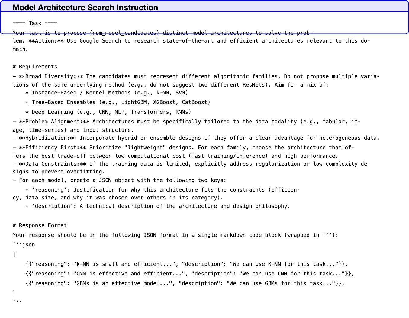
Text in this graphic
Model Architecture Search Instruction
⬇ ==== Task ==== Your task is to propose {num_model_candidates} distinct model architectures to solve the problem. Action: Use Google Search to research state-of-the-art and efficient architectures relevant to this domain. # Requirements - Broad Diversity: The candidates must represent different algorithmic families. Do not propose multiple variations of the same underlying method (e.g., do not suggest two different ResNets). Aim for a mix of: * Instance-Based / Kernel Methods (e.g., k-NN, SVM) * Tree-Based Ensembles (e.g., LightGBM, XGBoost, CatBoost) * Deep Learning (e.g., CNN, MLP, Transformers, RNNs) - Problem Alignment: Architectures must be specifically tailored to the data modality (e.g., tabular, image, time-series) and input structure. - Hybridization: Incorporate hybrid or ensemble designs if they offer a clear advantage for heterogeneous data. - Efficiency First: Prioritize "lightweight" designs. For each family, choose the architecture that offers the best trade-off between low computational cost (fast training/inference) and high performance. - Data Constraints: If the training data is limited, explicitly address regularization or low-complexity designs to prevent overfitting. - For each model, create a JSON object with the following two keys: - ‘reasoning‘: Justification for why this architecture fits the constraints (efficiency, data size, and why it was chosen over others in its category). - ‘description‘: A technical description of the architecture and design philosophy. # Response Format Your response should be in the following JSON format in a single markdown code block (wrapped in ‘‘‘): ‘‘‘json [ {{"reasoning": "k-NN is small and efficient...", "description": "We can use K-NN for this task..."}}, {{"reasoning": "CNN is effective and efficient...", "description": "We can use CNN for this task..."}}, {{"reasoning": "GBMs is an effective model...", "description": "We can use GBMs for this task..."}}, ] ‘‘‘
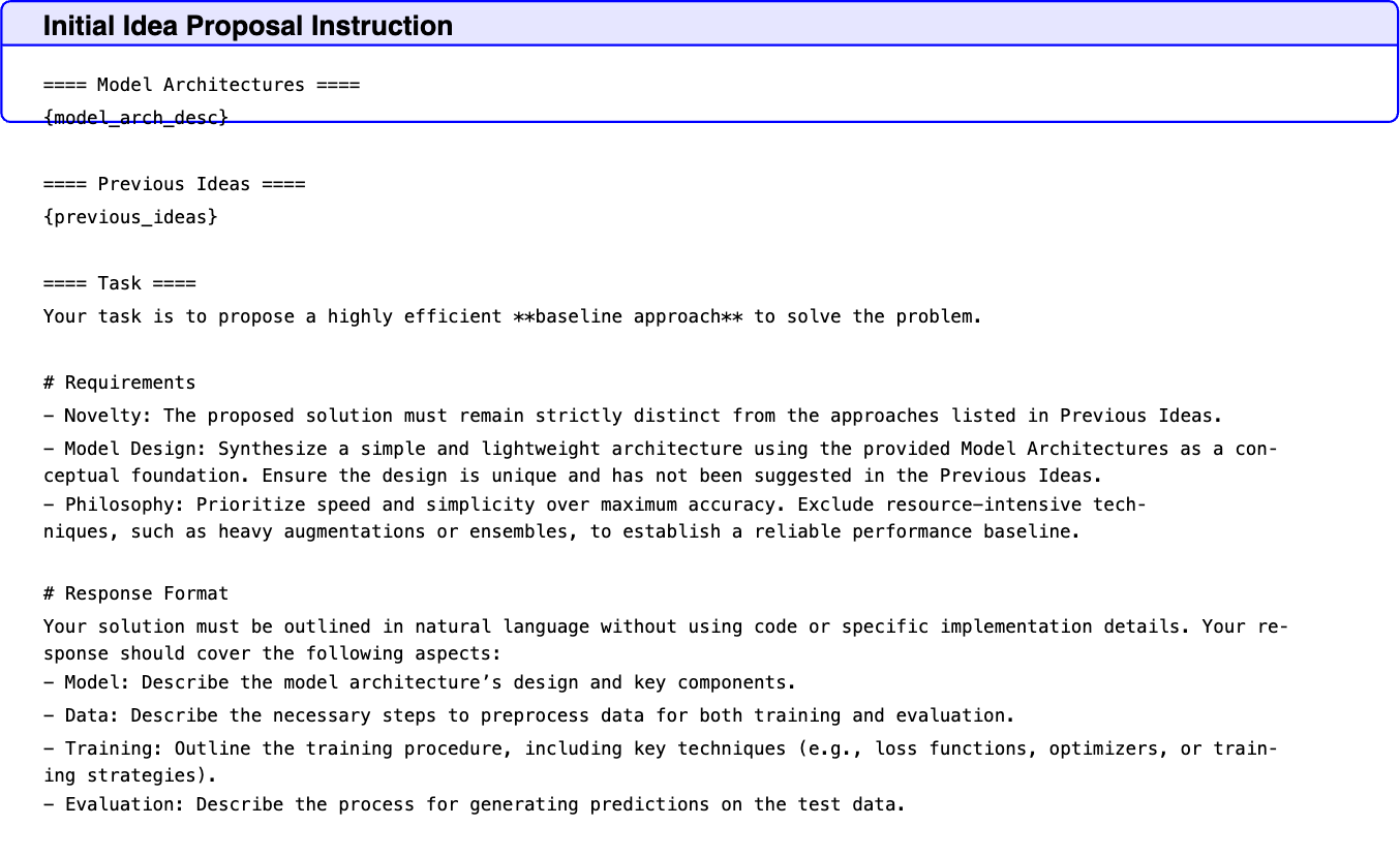
Text in this graphic
Initial Idea Proposal Instruction
⬇ ==== Model Architectures ==== {model_arch_desc} ==== Previous Ideas ==== {previous_ideas} ==== Task ==== Your task is to propose a highly efficient baseline approach to solve the problem. # Requirements - Novelty: The proposed solution must remain strictly distinct from the approaches listed in Previous Ideas. - Model Design: Synthesize a simple and lightweight architecture using the provided Model Architectures as a conceptual foundation. Ensure the design is unique and has not been suggested in the Previous Ideas. - Philosophy: Prioritize speed and simplicity over maximum accuracy. Exclude resource-intensive techniques, such as heavy augmentations or ensembles, to establish a reliable performance baseline. # Response Format Your solution must be outlined in natural language without using code or specific implementation details. Your response should cover the following aspects: - Model: Describe the model architecture’s design and key components. - Data: Describe the necessary steps to preprocess data for both training and evaluation. - Training: Outline the training procedure, including key techniques (e.g., loss functions, optimizers, or training strategies). - Evaluation: Describe the process for generating predictions on the test data.
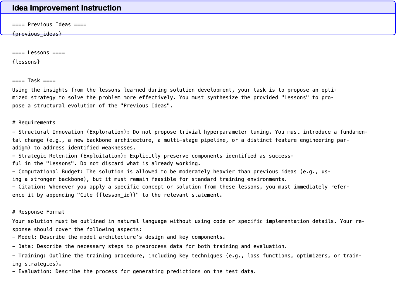
Text in this graphic
Idea Improvement Instruction
⬇ ==== Previous Ideas ==== {previous_ideas} ==== Lessons ==== {lessons} ==== Task ==== Using the insights from the lessons learned during solution development, your task is to propose an optimized strategy to solve the problem more effectively. You must synthesize the provided "Lessons" to propose a structural evolution of the "Previous Ideas". # Requirements - Structural Innovation (Exploration): Do not propose trivial hyperparameter tuning. You must introduce a fundamental change (e.g., a new backbone architecture, a multi-stage pipeline, or a distinct feature engineering paradigm) to address identified weaknesses. - Strategic Retention (Exploitation): Explicitly preserve components identified as successful in the "Lessons". Do not discard what is already working. - Computational Budget: The solution is allowed to be moderately heavier than previous ideas (e.g., using a stronger backbone), but it must remain feasible for standard training environments. - Citation: Whenever you apply a specific concept or solution from these lessons, you must immediately reference it by appending "Cite {{lesson_id}}" to the relevant statement. # Response Format Your solution must be outlined in natural language without using code or specific implementation details. Your response should cover the following aspects: - Model: Describe the model architecture’s design and key components. - Data: Describe the necessary steps to preprocess data for both training and evaluation. - Training: Outline the training procedure, including key techniques (e.g., loss functions, optimizers, or training strategies). - Evaluation: Describe the process for generating predictions on the test data.
Text in this graphic
Modular Decomposition Instruction
⬇ ==== Idea ==== {idea} ==== Task ==== Your task is to design a modular repository structure to implement the given idea. Do not generate the full code yet; focus on the natural description of the architectural logic. # Requirements - Modularity: Break the solution into logical modules based on functionality (e.g., data handling, core training and evaluation logic, utilities). - Entry Point: You must include a ‘main‘ module that acts as the entry point to execute the end-to-end pipeline. - Detail: For each module, the description must include: - The purpose of the module. - The names of specific classes or functions to be implemented. - A brief description of the implementation logic. - A brief explanation of how this module interacts with others. - Ordering: The JSON output must be ordered topologically (dependencies first, dependent modules last). # Response Format Provide the output strictly as a JSON object in a single markdown code block. The keys should be the module names and the values should be the detailed descriptions. The module name must not include the ‘.py‘ extension. Example Format: ‘‘‘json {{ "module_name": "Implements [Specific Class] to handle [Specific Task]. includes functions like [func_a] and [func_b].", "main": "Orchestrates the workflow. Imports DataLoader from the data module and Model from the model module to run the pipeline." }} ‘‘‘
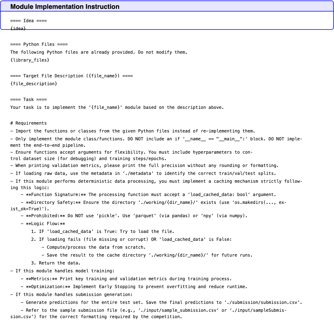
Text in this graphic
Module Implementation Instruction
⬇ ==== Idea ==== {idea} ==== Python Files ==== The following Python files are already provided. Do not modify them. {library_files} ==== Target File Description ({file_name}) ==== {file_description} ==== Task ==== Your task is to implement the ‘{file_name}‘ module based on the description above. # Requirements - Import the functions or classes from the given Python files instead of re-implementing them. - Only implement the module class/functions. DO NOT include an if ‘__name__ == "__main__":‘ block. DO NOT implement the end-to-end pipeline. - Ensure functions accept arguments for flexibility. You must include hyperparameters to control dataset size (for debugging) and training steps/epochs. - When printing validation metrics, please print the full precision without any rounding or formatting. - If loading raw data, use the metadata in ‘./metadata‘ to identify the correct train/val/test splits. - If this module performs deterministic data processing, you must implement a caching mechanism strictly following this logic: - Function Signature: The processing function must accept a ‘load_cached_data: bool‘ argument. - Directory Safety: Ensure the directory ‘./working/{dir_name}/‘ exists (use ‘os.makedirs(..., exist_ok=True)‘). - Prohibited: Do NOT use ‘pickle‘. Use ‘parquet‘ (via pandas) or ‘npy‘ (via numpy). - Logic Flow: 1. IF ‘load_cached_data‘ is True: Try to load the file. 2. IF loading fails (file missing or corrupt) OR ‘load_cached_data‘ is False: - Compute/process the data from scratch. - Save the result to the cache directory ‘./working/{dir_name}/‘ for future runs. 3. Return the data. - If this module handles model training: - Metrics: Print key training and validation metrics during training process. - Optimization: Implement Early Stopping to prevent overfitting and reduce runtime. - If this module handles submission generation: - Generate predictions for the entire test set. Save the final predictions to ‘./submission/submission.csv‘. - Refer to the sample submission file (e.g., ‘./input/sample_submission.csv‘ or ‘./input/sampleSubmission.csv‘) for the correct formatting required by the competition.
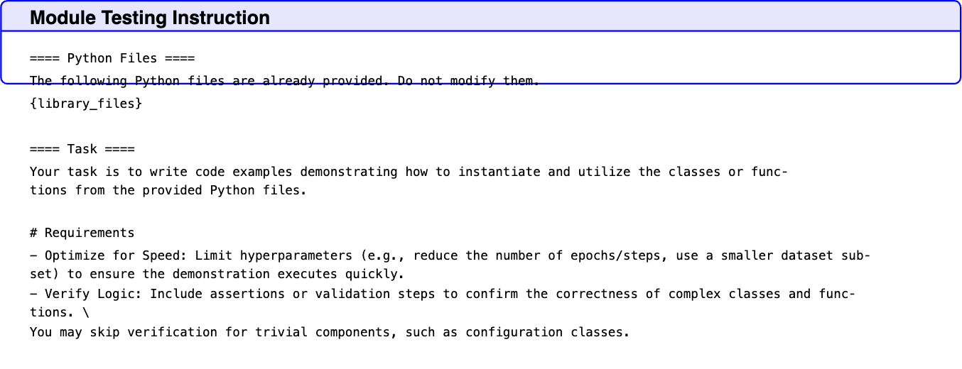
Text in this graphic
Module Testing Instruction
⬇ ==== Python Files ==== The following Python files are already provided. Do not modify them. {library_files} ==== Task ==== Your task is to write code examples demonstrating how to instantiate and utilize the classes or functions from the provided Python files. # Requirements - Optimize for Speed: Limit hyperparameters (e.g., reduce the number of epochs/steps, use a smaller dataset subset) to ensure the demonstration executes quickly. - Verify Logic: Include assertions or validation steps to confirm the correctness of complex classes and functions. \ You may skip verification for trivial components, such as configuration classes.
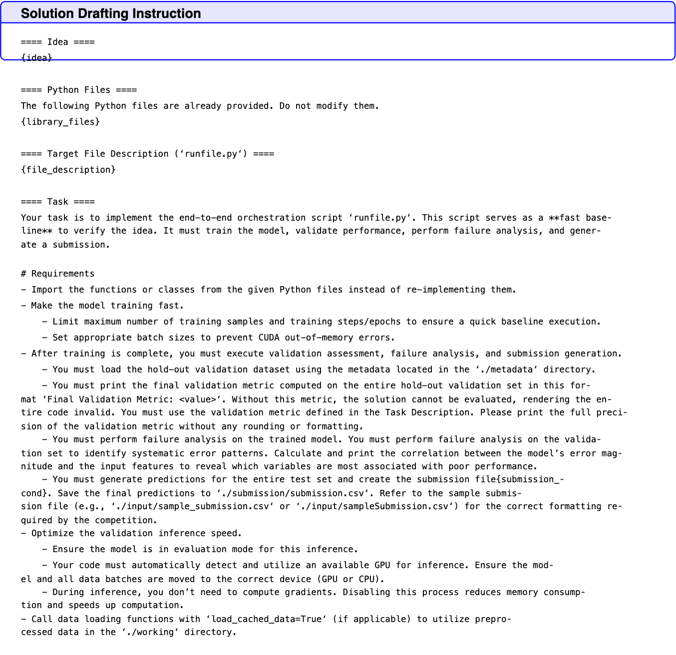
Text in this graphic
Solution Drafting Instruction
⬇ ==== Idea ==== {idea} ==== Python Files ==== The following Python files are already provided. Do not modify them. {library_files} ==== Target File Description (‘runfile.py‘) ==== {file_description} ==== Task ==== Your task is to implement the end-to-end orchestration script ‘runfile.py‘. This script serves as a fast baseline to verify the idea. It must train the model, validate performance, perform failure analysis, and generate a submission. # Requirements - Import the functions or classes from the given Python files instead of re-implementing them. - Make the model training fast. - Limit maximum number of training samples and training steps/epochs to ensure a quick baseline execution. - Set appropriate batch sizes to prevent CUDA out-of-memory errors. - After training is complete, you must execute validation assessment, failure analysis, and submission generation. - You must load the hold-out validation dataset using the metadata located in the ‘./metadata‘ directory. - You must print the final validation metric computed on the entire hold-out validation set in this format ‘Final Validation Metric: <value>‘. Without this metric, the solution cannot be evaluated, rendering the entire code invalid. You must use the validation metric defined in the Task Description. Please print the full precision of the validation metric without any rounding or formatting. - You must perform failure analysis on the trained model. You must perform failure analysis on the validation set to identify systematic error patterns. Calculate and print the correlation between the model’s error magnitude and the input features to reveal which variables are most associated with poor performance. - You must generate predictions for the entire test set and create the submission file{submission_cond}. Save the final predictions to ‘./submission/submission.csv‘. Refer to the sample submission file (e.g., ‘./input/sample_submission.csv‘ or ‘./input/sampleSubmission.csv‘) for the correct formatting required by the competition. - Optimize the validation inference speed. - Ensure the model is in evaluation mode for this inference. - Your code must automatically detect and utilize an available GPU for inference. Ensure the model and all data batches are moved to the correct device (GPU or CPU). - During inference, you don’t need to compute gradients. Disabling this process reduces memory consumption and speeds up computation. - Call data loading functions with ‘load_cached_data=True‘ (if applicable) to utilize preprocessed data in the ‘./working‘ directory.
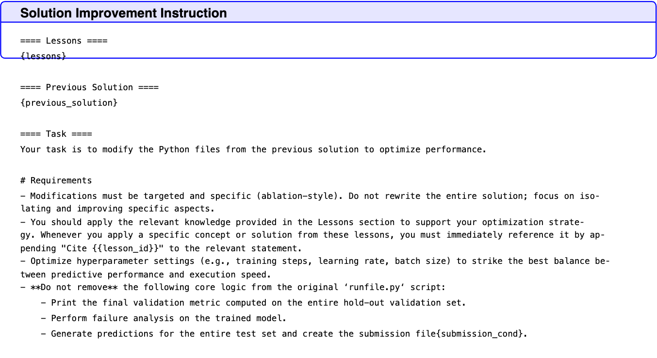
Text in this graphic
Solution Improvement Instruction
⬇ ==== Lessons ==== {lessons} ==== Previous Solution ==== {previous_solution} ==== Task ==== Your task is to modify the Python files from the previous solution to optimize performance. # Requirements - Modifications must be targeted and specific (ablation-style). Do not rewrite the entire solution; focus on isolating and improving specific aspects. - You should apply the relevant knowledge provided in the Lessons section to support your optimization strategy. Whenever you apply a specific concept or solution from these lessons, you must immediately reference it by appending "Cite {{lesson_id}}" to the relevant statement. - Optimize hyperparameter settings (e.g., training steps, learning rate, batch size) to strike the best balance between predictive performance and execution speed. - Do not remove the following core logic from the original ‘runfile.py‘ script: - Print the final validation metric computed on the entire hold-out validation set. - Perform failure analysis on the trained model. - Generate predictions for the entire test set and create the submission file{submission_cond}.
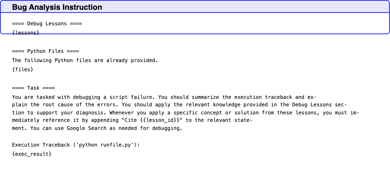
Text in this graphic
Bug Analysis Instruction
⬇ ==== Debug Lessons ==== {lessons} ==== Python Files ==== The following Python files are already provided. {files} ==== Task ==== You are tasked with debugging a script failure. You should summarize the execution traceback and explain the root cause of the errors. You should apply the relevant knowledge provided in the Debug Lessons section to support your diagnosis. Whenever you apply a specific concept or solution from these lessons, you must immediately reference it by appending "Cite {{lesson_id}}" to the relevant statement. You can use Google Search as needed for debugging. Execution Traceback (‘python runfile.py‘): {exec_result}
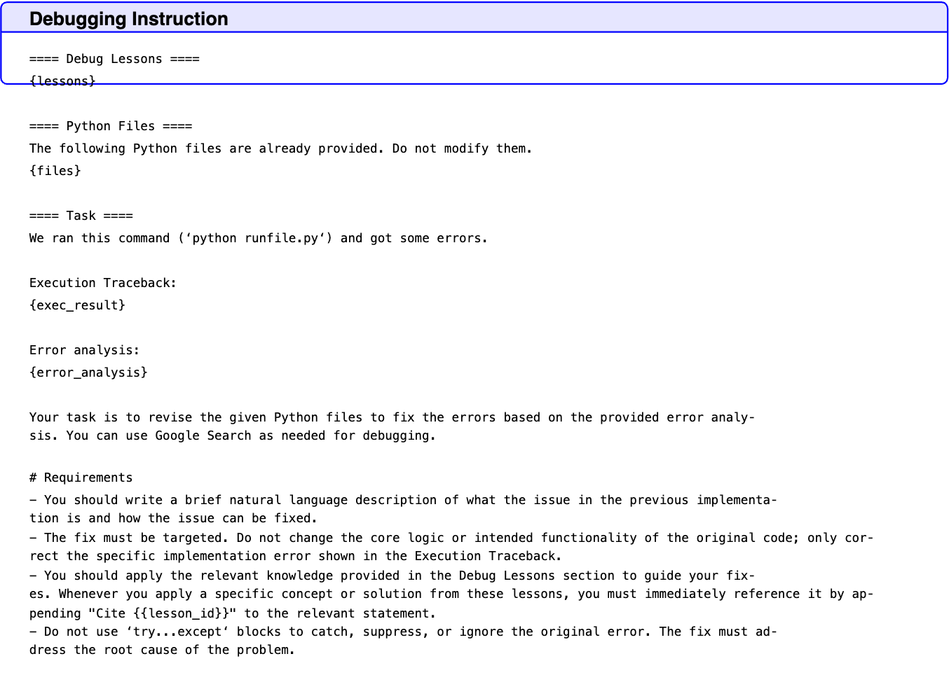
Text in this graphic
Debugging Instruction
⬇ ==== Debug Lessons ==== {lessons} ==== Python Files ==== The following Python files are already provided. Do not modify them. {files} ==== Task ==== We ran this command (‘python runfile.py‘) and got some errors. Execution Traceback: {exec_result} Error analysis: {error_analysis} Your task is to revise the given Python files to fix the errors based on the provided error analysis. You can use Google Search as needed for debugging. # Requirements - You should write a brief natural language description of what the issue in the previous implementation is and how the issue can be fixed. - The fix must be targeted. Do not change the core logic or intended functionality of the original code; only correct the specific implementation error shown in the Execution Traceback. - You should apply the relevant knowledge provided in the Debug Lessons section to guide your fixes. Whenever you apply a specific concept or solution from these lessons, you must immediately reference it by appending "Cite {{lesson_id}}" to the relevant statement. - Do not use ‘try...except‘ blocks to catch, suppress, or ignore the original error. The fix must address the root cause of the problem.
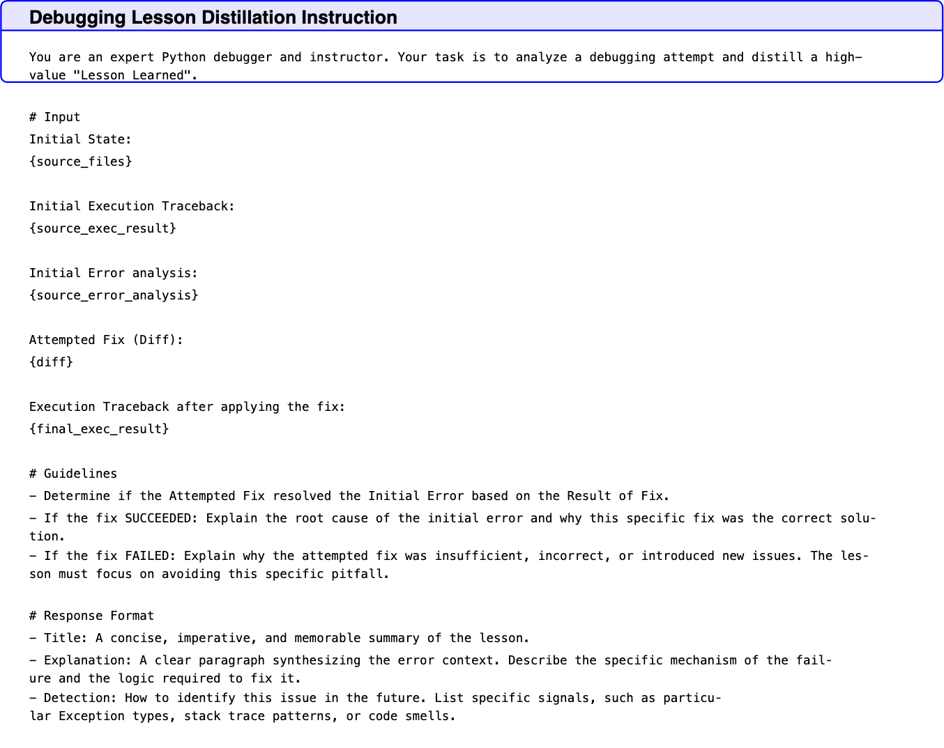
Text in this graphic
Debugging Lesson Distillation Instruction
⬇ You are an expert Python debugger and instructor. Your task is to analyze a debugging attempt and distill a high-value "Lesson Learned". # Input Initial State: {source_files} Initial Execution Traceback: {source_exec_result} Initial Error analysis: {source_error_analysis} Attempted Fix (Diff): {diff} Execution Traceback after applying the fix: {final_exec_result} # Guidelines - Determine if the Attempted Fix resolved the Initial Error based on the Result of Fix. - If the fix SUCCEEDED: Explain the root cause of the initial error and why this specific fix was the correct solution. - If the fix FAILED: Explain why the attempted fix was insufficient, incorrect, or introduced new issues. The lesson must focus on avoiding this specific pitfall. # Response Format - Title: A concise, imperative, and memorable summary of the lesson. - Explanation: A clear paragraph synthesizing the error context. Describe the specific mechanism of the failure and the logic required to fix it. - Detection: How to identify this issue in the future. List specific signals, such as particular Exception types, stack trace patterns, or code smells.
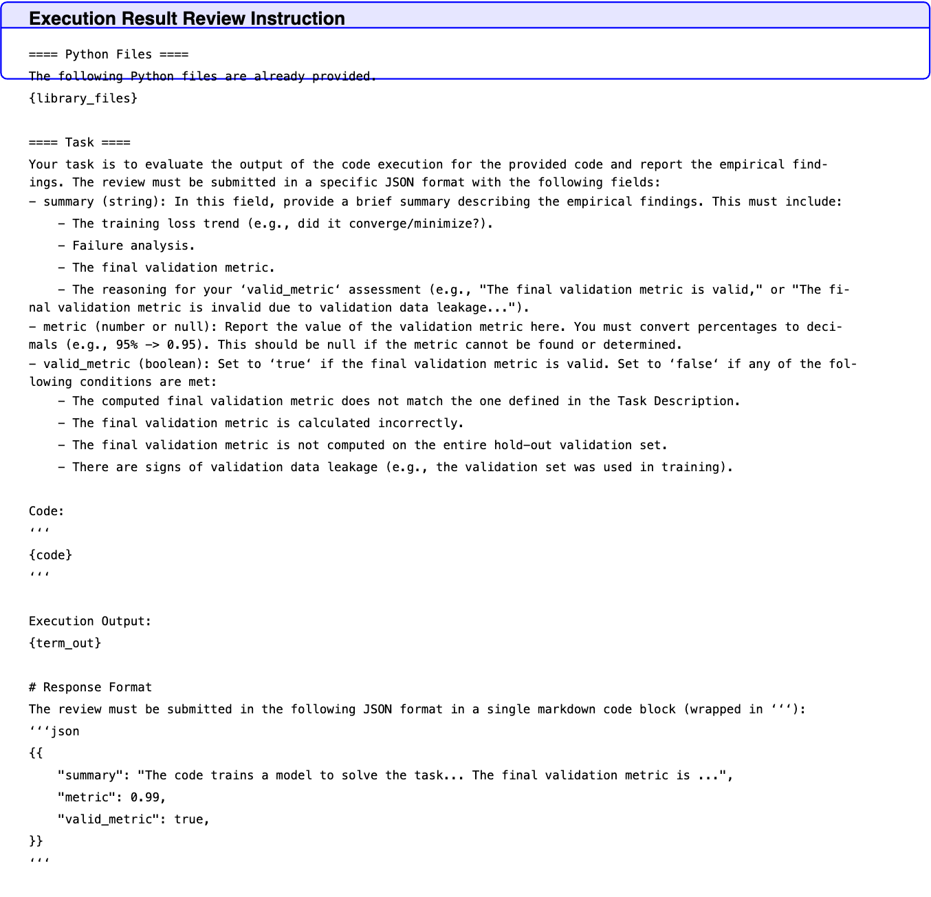
Text in this graphic
Execution Result Review Instruction
⬇ ==== Python Files ==== The following Python files are already provided. {library_files} ==== Task ==== Your task is to evaluate the output of the code execution for the provided code and report the empirical findings. The review must be submitted in a specific JSON format with the following fields: - summary (string): In this field, provide a brief summary describing the empirical findings. This must include: - The training loss trend (e.g., did it converge/minimize?). - Failure analysis. - The final validation metric. - The reasoning for your ‘valid_metric‘ assessment (e.g., "The final validation metric is valid," or "The final validation metric is invalid due to validation data leakage..."). - metric (number or null): Report the value of the validation metric here. You must convert percentages to decimals (e.g., 95% -> 0.95). This should be null if the metric cannot be found or determined. - valid_metric (boolean): Set to ‘true‘ if the final validation metric is valid. Set to ‘false‘ if any of the following conditions are met: - The computed final validation metric does not match the one defined in the Task Description. - The final validation metric is calculated incorrectly. - The final validation metric is not computed on the entire hold-out validation set. - There are signs of validation data leakage (e.g., the validation set was used in training). Code: ‘‘‘ {code} ‘‘‘ Execution Output: {term_out} # Response Format The review must be submitted in the following JSON format in a single markdown code block (wrapped in ‘‘‘): ‘‘‘json {{ "summary": "The code trains a model to solve the task... The final validation metric is ...", "metric": 0.99, "valid_metric": true, }} ‘‘‘
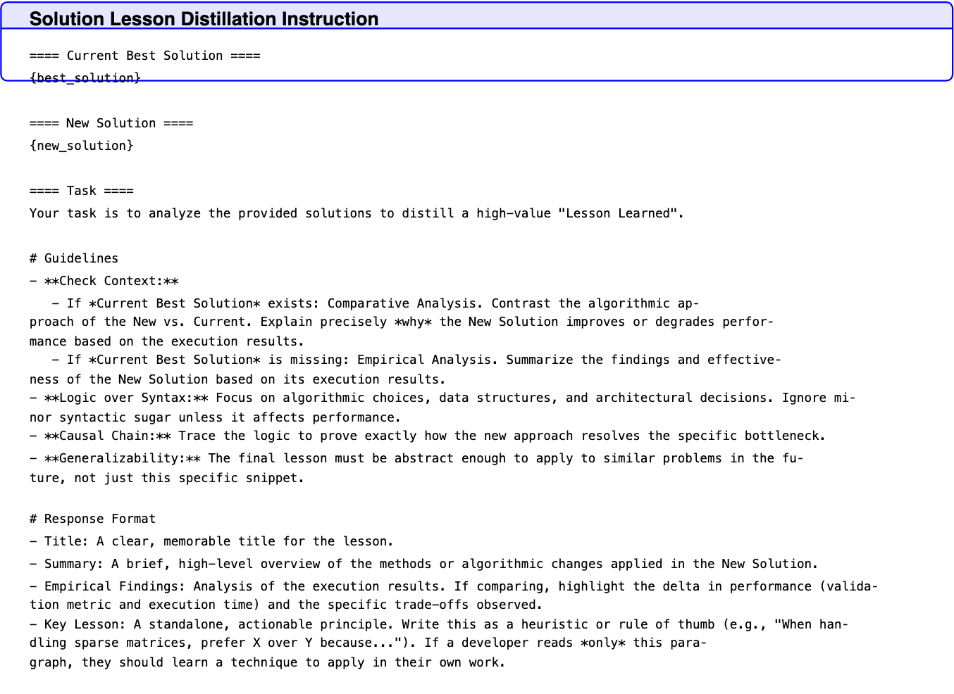
Text in this graphic
Solution Lesson Distillation Instruction
⬇ ==== Current Best Solution ==== {best_solution} ==== New Solution ==== {new_solution} ==== Task ==== Your task is to analyze the provided solutions to distill a high-value "Lesson Learned". # Guidelines - Check Context: - If *Current Best Solution* exists: Comparative Analysis. Contrast the algorithmic approach of the New vs. Current. Explain precisely *why* the New Solution improves or degrades performance based on the execution results. - If *Current Best Solution* is missing: Empirical Analysis. Summarize the findings and effectiveness of the New Solution based on its execution results. - Logic over Syntax: Focus on algorithmic choices, data structures, and architectural decisions. Ignore minor syntactic sugar unless it affects performance. - Causal Chain: Trace the logic to prove exactly how the new approach resolves the specific bottleneck. - Generalizability: The final lesson must be abstract enough to apply to similar problems in the future, not just this specific snippet. # Response Format - Title: A clear, memorable title for the lesson. - Summary: A brief, high-level overview of the methods or algorithmic changes applied in the New Solution. - Empirical Findings: Analysis of the execution results. If comparing, highlight the delta in performance (validation metric and execution time) and the specific trade-offs observed. - Key Lesson: A standalone, actionable principle. Write this as a heuristic or rule of thumb (e.g., "When handling sparse matrices, prefer X over Y because..."). If a developer reads *only* this paragraph, they should learn a technique to apply in their own work.
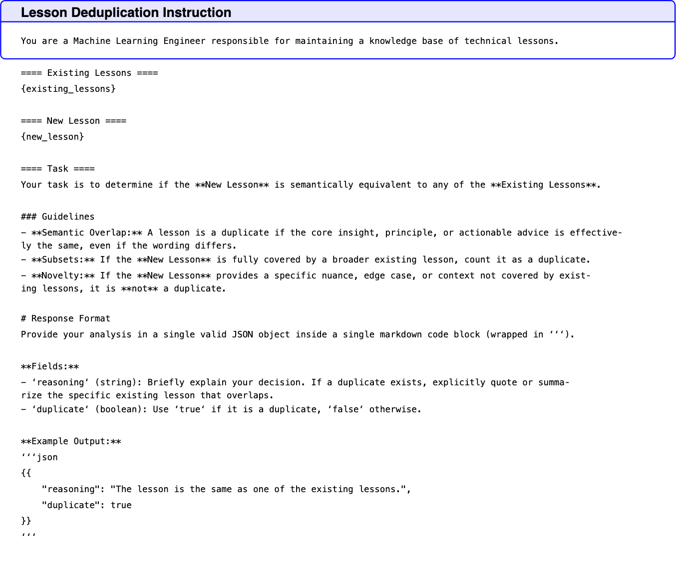
Text in this graphic
Lesson Deduplication Instruction
⬇ You are a Machine Learning Engineer responsible for maintaining a knowledge base of technical lessons. ==== Existing Lessons ==== {existing_lessons} ==== New Lesson ==== {new_lesson} ==== Task ==== Your task is to determine if the New Lesson is semantically equivalent to any of the Existing Lessons. ### Guidelines - Semantic Overlap: A lesson is a duplicate if the core insight, principle, or actionable advice is effectively the same, even if the wording differs. - Subsets: If the New Lesson is fully covered by a broader existing lesson, count it as a duplicate. - Novelty: If the New Lesson provides a specific nuance, edge case, or context not covered by existing lessons, it is not a duplicate. # Response Format Provide your analysis in a single valid JSON object inside a single markdown code block (wrapped in ‘‘‘). Fields: - ‘reasoning‘ (string): Briefly explain your decision. If a duplicate exists, explicitly quote or summarize the specific existing lesson that overlaps. - ‘duplicate‘ (boolean): Use ‘true‘ if it is a duplicate, ‘false‘ otherwise. Example Output: ‘‘‘json {{ "reasoning": "The lesson is the same as one of the existing lessons.", "duplicate": true }} ‘‘‘
In this section, we showcase the final solution generated for the iMet-2020-fgvc7 competition. This repository was produced by MARS utilizing Gemini-3-Pro-Preview and achieved the highest validation performance during the search process.
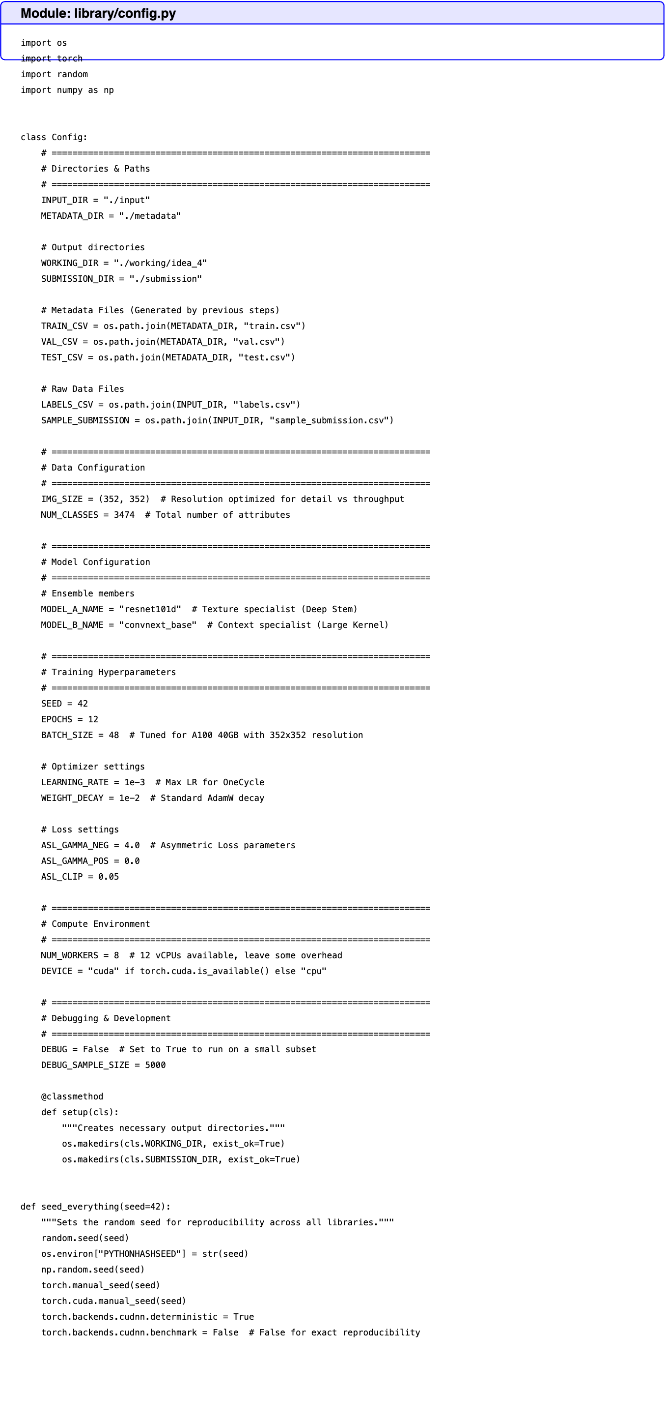
Text in this graphic
Module: library/config.py
⬇ import os import torch import random import numpy as np class Config: # ========================================================================= # Directories & Paths # ========================================================================= INPUT_DIR = "./input" METADATA_DIR = "./metadata" # Output directories WORKING_DIR = "./working/idea_4" SUBMISSION_DIR = "./submission" # Metadata Files (Generated by previous steps) TRAIN_CSV = os.path.join(METADATA_DIR, "train.csv") VAL_CSV = os.path.join(METADATA_DIR, "val.csv") TEST_CSV = os.path.join(METADATA_DIR, "test.csv") # Raw Data Files LABELS_CSV = os.path.join(INPUT_DIR, "labels.csv") SAMPLE_SUBMISSION = os.path.join(INPUT_DIR, "sample_submission.csv") # ========================================================================= # Data Configuration # ========================================================================= IMG_SIZE = (352, 352) # Resolution optimized for detail vs throughput NUM_CLASSES = 3474 # Total number of attributes # ========================================================================= # Model Configuration # ========================================================================= # Ensemble members MODEL_A_NAME = "resnet101d" # Texture specialist (Deep Stem) MODEL_B_NAME = "convnext_base" # Context specialist (Large Kernel) # ========================================================================= # Training Hyperparameters # ========================================================================= SEED = 42 EPOCHS = 12 BATCH_SIZE = 48 # Tuned for A100 40GB with 352x352 resolution # Optimizer settings LEARNING_RATE = 1e-3 # Max LR for OneCycle WEIGHT_DECAY = 1e-2 # Standard AdamW decay # Loss settings ASL_GAMMA_NEG = 4.0 # Asymmetric Loss parameters ASL_GAMMA_POS = 0.0 ASL_CLIP = 0.05 # ========================================================================= # Compute Environment # ========================================================================= NUM_WORKERS = 8 # 12 vCPUs available, leave some overhead DEVICE = "cuda" if torch.cuda.is_available() else "cpu" # ========================================================================= # Debugging & Development # ========================================================================= DEBUG = False # Set to True to run on a small subset DEBUG_SAMPLE_SIZE = 5000 @classmethod def setup(cls): """Creates necessary output directories.""" os.makedirs(cls.WORKING_DIR, exist_ok=True) os.makedirs(cls.SUBMISSION_DIR, exist_ok=True) def seed_everything(seed=42): """Sets the random seed for reproducibility across all libraries.""" random.seed(seed) os.environ["PYTHONHASHSEED"] = str(seed) np.random.seed(seed) torch.manual_seed(seed) torch.cuda.manual_seed(seed) torch.backends.cudnn.deterministic = True torch.backends.cudnn.benchmark = False # False for exact reproducibility # Initialize directories on import Config.setup()

Text in this graphic
Module: library/dataset.py
⬇ import os import cv2 import torch import numpy as np import pandas as pd import albumentations as A from albumentations.pytorch import ToTensorV2 from torch.utils.data import Dataset, DataLoader from library.config import Config def load_processed_dataframe(mode, load_cached_data=True): """ Loads the metadata dataframe for a specific mode (train/val/test). Implements caching using Parquet files to store processed dataframes (where attribute_ids strings are converted to lists). """ cache_dir = Config.WORKING_DIR os.makedirs(cache_dir, exist_ok=True) cache_path = os.path.join(cache_dir, f"cached_{mode}.parquet") # 1. Try to load from cache if load_cached_data and os.path.exists(cache_path): try: df = pd.read_parquet(cache_path) return df except Exception: # If load fails, proceed to process from scratch pass # 2. Process from scratch if mode == "train": csv_path = Config.TRAIN_CSV elif mode == "val": csv_path = Config.VAL_CSV elif mode == "test": csv_path = Config.TEST_CSV else: raise ValueError(f"Unknown mode: {mode}") if not os.path.exists(csv_path): raise FileNotFoundError(f"Metadata file not found: {csv_path}") df = pd.read_csv(csv_path) # Parse attribute_ids: "0 1 2" -> [0, 1, 2] # Handle NaNs by converting to empty string first df["attribute_ids"] = df["attribute_ids"].fillna("") # Function to safe convert string to list of ints def parse_ids(x): if not x.strip(): return np.array([], dtype=int) return np.array([int(i) for i in x.split()], dtype=int) # We store as numpy arrays inside the dataframe cells for parquet compatibility/efficiency df["parsed_attributes"] = df["attribute_ids"].apply(parse_ids) # 3. Save to cache try: df.to_parquet(cache_path, index=False) except Exception as e: print(f"Warning: Failed to save cache to {cache_path}: {e}") return df class ArtworkDataset(Dataset): def __init__(self, df, transforms=None, mode="train"): """ Args: df (pd.DataFrame): DataFrame containing metadata. transforms (albumentations.Compose): Transforms to apply. mode (str): ’train’, ’val’, or ’test’. """ self.df = df self.transforms = transforms self.mode = mode self.input_dir = Config.INPUT_DIR self.num_classes = Config.NUM_CLASSES def __len__(self): return len(self.df) def __getitem__(self, idx): row = self.df.iloc[idx] image_id = row["id"] file_path = row["file_path"] # Load Image full_path = os.path.join(self.input_dir, file_path) image = cv2.imread(full_path) if image is None: # Fallback for missing/corrupt images: return black image # This prevents crashing during training image = np.zeros( (Config.IMG_SIZE[0], Config.IMG_SIZE[1], 3), dtype=np.uint8 ) else: image = cv2.cvtColor(image, cv2.COLOR_BGR2RGB) # Apply Transforms if self.transforms: augmented = self.transforms(image=image) image = augmented["image"] # Create Target (Multi-hot encoding) target = torch.zeros(self.num_classes, dtype=torch.float32) # In test mode, we might not have valid labels, but we still return a dummy target # parsed_attributes is a numpy array of integers attr_ids = row["parsed_attributes"] if len(attr_ids) > 0: # Ensure indices are within bounds valid_ids = attr_ids[attr_ids < self.num_classes] target[valid_ids] = 1.0 return image, target, image_id def get_transforms(mode="train"): """ Returns the Albumentations transform pipeline for the specified mode. """ img_size = Config.IMG_SIZE if mode == "train": return A.Compose( [ A.Resize(height=img_size[0], width=img_size[1]), A.HorizontalFlip(p=0.5), A.Normalize( mean=(0.485, 0.456, 0.406), std=(0.229, 0.224, 0.225), max_pixel_value=255.0, p=1.0, ), ToTensorV2(), ] ) else: # Validation and Test return A.Compose( [ A.Resize(height=img_size[0], width=img_size[1]), A.Normalize( mean=(0.485, 0.456, 0.406), std=(0.229, 0.224, 0.225), max_pixel_value=255.0, p=1.0, ), ToTensorV2(), ] ) def get_dataloaders( debug=False, batch_size=Config.BATCH_SIZE, num_workers=Config.NUM_WORKERS, load_cached_data=True, ): """ Creates and returns DataLoaders for train, validation, and test sets. Args: debug (bool): If True, subsets the data for quick debugging. batch_size (int): Batch size for the dataloaders. num_workers (int): Number of worker processes. load_cached_data (bool): Whether to use cached dataframes. Returns: tuple: (train_loader, val_loader, test_loader) """ # Load DataFrames train_df = load_processed_dataframe("train", load_cached_data) val_df = load_processed_dataframe("val", load_cached_data) test_df = load_processed_dataframe("test", load_cached_data) # Debug Subsampling if debug: debug_size = Config.DEBUG_SAMPLE_SIZE train_df = train_df.iloc[:debug_size] val_df = val_df.iloc[:debug_size] test_df = test_df.iloc[:debug_size] # Create Datasets train_dataset = ArtworkDataset( train_df, transforms=get_transforms("train"), mode="train" ) val_dataset = ArtworkDataset(val_df, transforms=get_transforms("val"), mode="val") test_dataset = ArtworkDataset( test_df, transforms=get_transforms("test"), mode="test" ) # Create DataLoaders train_loader = DataLoader( train_dataset, batch_size=batch_size, shuffle=True, num_workers=num_workers, pin_memory=True, drop_last=True, ) val_loader = DataLoader( val_dataset, batch_size=batch_size, shuffle=False, num_workers=num_workers, pin_memory=True, drop_last=False, ) test_loader = DataLoader( test_dataset, batch_size=batch_size, shuffle=False, num_workers=num_workers, pin_memory=True, drop_last=False, ) return train_loader, val_loader, test_loader

Text in this graphic
Module: library/inference.py
⬇ import os import torch import numpy as np import pandas as pd from tqdm import tqdm from library.config import Config from library.dataset import get_dataloaders from library.models import get_model from library.utils import optimize_threshold, load_checkpoint def predict_with_tta(model, dataloader, device, mode="val"): """ Generates predictions using Test Time Augmentation (Horizontal Flip). Args: model (nn.Module): The trained model. dataloader (DataLoader): DataLoader for validation or test set. device (torch.device): Device to run inference on. mode (str): ’val’ or ’test’. Returns: tuple: (all_probs, all_targets_or_ids) - all_probs: np.ndarray of shape (N, num_classes) - all_targets_or_ids: np.ndarray of targets (if val) or list of ids (if test) """ model.eval() all_probs = [] all_targets_or_ids = [] with torch.no_grad(): for batch in dataloader: images, targets, ids = batch images = images.to(device) # 1. Forward pass original out_orig = model(images) probs_orig = torch.sigmoid(out_orig) # 2. Forward pass flipped (TTA) # Flip along width dimension (dim 3 for NCHW) images_flipped = torch.flip(images, dims=[3]) out_flipped = model(images_flipped) probs_flipped = torch.sigmoid(out_flipped) # 3. Average probabilities avg_probs = (probs_orig + probs_flipped) / 2.0 all_probs.append(avg_probs.cpu().numpy()) # Collect targets or IDs based on mode if mode == "test": all_targets_or_ids.extend(ids) else: all_targets_or_ids.append(targets.numpy()) all_probs = np.concatenate(all_probs, axis=0) if mode != "test": all_targets_or_ids = np.concatenate(all_targets_or_ids, axis=0) return all_probs, all_targets_or_ids def get_model_predictions(model_name, mode, dataloader, device, load_cached_data=True): """ Gets predictions for a specific model and mode (val/test). Implements caching of the raw probability arrays. Args: model_name (str): Name of the model architecture. mode (str): ’val’ or ’test’. dataloader (DataLoader): The data loader. device (torch.device): Compute device. load_cached_data (bool): Whether to use cached .npy files. Returns: tuple: (probs, targets_or_ids) """ cache_dir = Config.WORKING_DIR os.makedirs(cache_dir, exist_ok=True) probs_path = os.path.join(cache_dir, f"{model_name}_{mode}_probs.npy") meta_path = os.path.join( cache_dir, f"{model_name}_{mode}_meta.npy" ) # targets or ids # Try to load from cache if load_cached_data and os.path.exists(probs_path) and os.path.exists(meta_path): print(f"Loading cached predictions for {model_name} ({mode})...") try: probs = np.load(probs_path) meta = np.load(meta_path, allow_pickle=True) if len(probs) != len(dataloader.dataset): raise ValueError( f"Cache size mismatch: {len(probs)} vs {len(dataloader.dataset)}" ) return probs, meta except Exception as e: print(f"Failed to load cache: {e}. Re-running inference.") # Run inference print(f"Running inference for {model_name} ({mode})...") # Load model and checkpoint model = get_model(model_name, num_classes=Config.NUM_CLASSES, pretrained=False) model = model.to(device) checkpoint_filename = f"{model_name}_best.pth" try: load_checkpoint(model, checkpoint_filename, device=device) except FileNotFoundError: print( f"Warning: Checkpoint {checkpoint_filename} not found. Using random weights (for debugging only)." ) probs, meta = predict_with_tta(model, dataloader, device, mode=mode) # Save to cache np.save(probs_path, probs) np.save(meta_path, meta) # Clean up del model torch.cuda.empty_cache() return probs, meta def ensemble_predictions(probs_list): """ Averages a list of probability arrays. """ if not probs_list: return None return np.mean(probs_list, axis=0) def generate_submission(debug=Config.DEBUG, load_cached_data=True): """ Main function to generate the submission file. 1. Loads Val and Test loaders. 2. Gets predictions for Model A and Model B (with TTA). 3. Ensembles predictions. 4. Optimizes threshold on Validation set. 5. Applies threshold to Test set. 6. Saves submission.csv. """ device = torch.device(Config.DEVICE) # 1. Get DataLoaders # We don’t need the train loader here _, val_loader, test_loader = get_dataloaders( debug=debug, batch_size=Config.BATCH_SIZE, num_workers=Config.NUM_WORKERS, load_cached_data=load_cached_data, ) models = [Config.MODEL_A_NAME, Config.MODEL_B_NAME] # 2. Validation Inference (for Threshold Calibration) print("--- Processing Validation Set ---") val_probs_list = [] val_targets = None for model_name in models: probs, targets = get_model_predictions( model_name, "val", val_loader, device, load_cached_data ) val_probs_list.append(probs) val_targets = targets # Targets should be same for all models # Ensemble Validation val_ensemble_probs = ensemble_predictions(val_probs_list) # Optimize Threshold print("Optimizing threshold on ensemble...") best_threshold, best_score = optimize_threshold(val_targets, val_ensemble_probs) print(f"Optimal Threshold: {best_threshold}") print(f"Validation Micro-F1 Score with Optimal Threshold: {best_score}") # 3. Test Inference print("\n--- Processing Test Set ---") test_probs_list = [] test_ids = None for model_name in models: probs, ids = get_model_predictions( model_name, "test", test_loader, device, load_cached_data ) test_probs_list.append(probs) test_ids = ids # IDs should be same for all models # Ensemble Test test_ensemble_probs = ensemble_predictions(test_probs_list) # 4. Generate Submission CSV print(f"Generating submission with threshold {best_threshold}...") # Binarize predictions predictions_bin = (test_ensemble_probs > best_threshold).astype(int) submission_rows = [] for idx, image_id in enumerate(test_ids): # Get indices of positive classes pred_indices = np.where(predictions_bin[idx] == 1)[0] # Format as space-separated string pred_str = " ".join(map(str, pred_indices)) submission_rows.append({"id": image_id, "attribute_ids": pred_str}) submission_df = pd.DataFrame(submission_rows) # Save out_path = os.path.join(Config.SUBMISSION_DIR, "submission.csv") submission_df.to_csv(out_path, index=False) print(f"Submission saved to {out_path}") return best_score
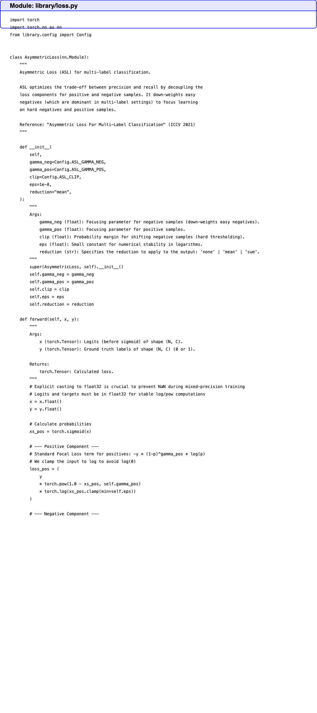
Text in this graphic
Module: library/loss.py
⬇ import torch import torch.nn as nn from library.config import Config class AsymmetricLoss(nn.Module): """ Asymmetric Loss (ASL) for multi-label classification. ASL optimizes the trade-off between precision and recall by decoupling the loss components for positive and negative samples. It down-weights easy negatives (which are dominant in multi-label settings) to focus learning on hard negatives and positive samples. Reference: "Asymmetric Loss For Multi-Label Classification" (ICCV 2021) """ def __init__( self, gamma_neg=Config.ASL_GAMMA_NEG, gamma_pos=Config.ASL_GAMMA_POS, clip=Config.ASL_CLIP, eps=1e-8, reduction="mean", ): """ Args: gamma_neg (float): Focusing parameter for negative samples (down-weights easy negatives). gamma_pos (float): Focusing parameter for positive samples. clip (float): Probability margin for shifting negative samples (hard thresholding). eps (float): Small constant for numerical stability in logarithms. reduction (str): Specifies the reduction to apply to the output: ’none’ | ’mean’ | ’sum’. """ super(AsymmetricLoss, self).__init__() self.gamma_neg = gamma_neg self.gamma_pos = gamma_pos self.clip = clip self.eps = eps self.reduction = reduction def forward(self, x, y): """ Args: x (torch.Tensor): Logits (before sigmoid) of shape (N, C). y (torch.Tensor): Ground truth labels of shape (N, C) (0 or 1). Returns: torch.Tensor: Calculated loss. """ # Explicit casting to float32 is crucial to prevent NaN during mixed-precision training # Logits and targets must be in float32 for stable log/pow computations x = x.float() y = y.float() # Calculate probabilities xs_pos = torch.sigmoid(x) # --- Positive Component --- # Standard Focal Loss term for positives: -y * (1-p)^gamma_pos * log(p) # We clamp the input to log to avoid log(0) loss_pos = ( y * torch.pow(1.0 - xs_pos, self.gamma_pos) * torch.log(xs_pos.clamp(min=self.eps)) ) # --- Negative Component --- # ASL modification: Shifted probability for negatives # p_m = max(p - clip, 0) # This hard-thresholds easy negatives (where p < clip) to have 0 loss and 0 gradient xs_neg = xs_pos if self.clip > 0: xs_neg = (xs_neg - self.clip).clamp(min=0) # Negative term: -(1-y) * (p_m)^gamma_neg * log(1 - p_m) loss_neg = ( (1.0 - y) * torch.pow(xs_neg, self.gamma_neg) * torch.log((1.0 - xs_neg).clamp(min=self.eps)) ) # Combine components # Note: The negative signs from the formulas are applied here loss = -(loss_pos + loss_neg) # Apply reduction if self.reduction == "mean": return loss.mean() elif self.reduction == "sum": return loss.sum() else: return loss
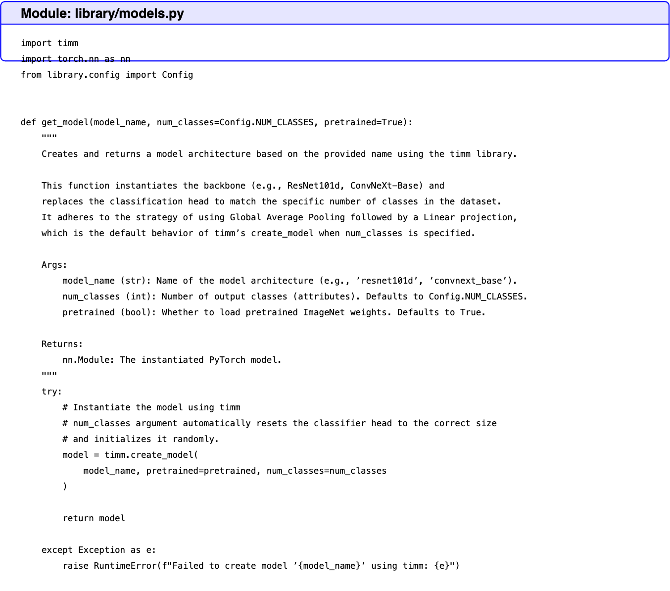
Text in this graphic
Module: library/models.py
⬇ import timm import torch.nn as nn from library.config import Config def get_model(model_name, num_classes=Config.NUM_CLASSES, pretrained=True): """ Creates and returns a model architecture based on the provided name using the timm library. This function instantiates the backbone (e.g., ResNet101d, ConvNeXt-Base) and replaces the classification head to match the specific number of classes in the dataset. It adheres to the strategy of using Global Average Pooling followed by a Linear projection, which is the default behavior of timm’s create_model when num_classes is specified. Args: model_name (str): Name of the model architecture (e.g., ’resnet101d’, ’convnext_base’). num_classes (int): Number of output classes (attributes). Defaults to Config.NUM_CLASSES. pretrained (bool): Whether to load pretrained ImageNet weights. Defaults to True. Returns: nn.Module: The instantiated PyTorch model. """ try: # Instantiate the model using timm # num_classes argument automatically resets the classifier head to the correct size # and initializes it randomly. model = timm.create_model( model_name, pretrained=pretrained, num_classes=num_classes ) return model except Exception as e: raise RuntimeError(f"Failed to create model ’{model_name}’ using timm: {e}")

Text in this graphic
Module: library/train.py
⬇ import os import time import torch import torch.nn as nn import torch.optim as optim import numpy as np from torch.cuda.amp import GradScaler, autocast from torch.optim.lr_scheduler import OneCycleLR from library.config import Config, seed_everything from library.dataset import get_dataloaders from library.models import get_model from library.loss import AsymmetricLoss from library.utils import calculate_f1_score, optimize_threshold, save_checkpoint class Trainer: """ Manages the training and validation process for a single model. """ def __init__(self, model, optimizer, scheduler, criterion, device, scaler): self.model = model self.optimizer = optimizer self.scheduler = scheduler self.criterion = criterion self.device = device self.scaler = scaler self.best_score = 0.0 def train_epoch(self, train_loader, epoch): """ Runs one epoch of training. """ self.model.train() running_loss = 0.0 num_batches = len(train_loader) for i, (images, targets, _) in enumerate(train_loader): images = images.to(self.device, non_blocking=True) targets = targets.to(self.device, non_blocking=True) self.optimizer.zero_grad() # Mixed precision training with autocast(): outputs = self.model(images) loss = self.criterion(outputs, targets) self.scaler.scale(loss).backward() self.scaler.step(self.optimizer) self.scaler.update() if self.scheduler is not None: self.scheduler.step() running_loss += loss.item() avg_loss = running_loss / num_batches return avg_loss def validate(self, val_loader): """ Runs validation and calculates metrics. """ self.model.eval() running_loss = 0.0 all_preds = [] all_targets = [] with torch.no_grad(): for images, targets, _ in val_loader: images = images.to(self.device, non_blocking=True) targets = targets.to(self.device, non_blocking=True) # Mixed precision inference with autocast(): outputs = self.model(images) loss = self.criterion(outputs, targets) running_loss += loss.item() # Apply sigmoid for probabilities probs = torch.sigmoid(outputs) all_preds.append(probs.cpu().numpy()) all_targets.append(targets.cpu().numpy()) avg_loss = running_loss / len(val_loader) all_preds = np.concatenate(all_preds, axis=0) all_targets = np.concatenate(all_targets, axis=0) # Calculate F1 Score (Standard 0.5 threshold) f1_score = calculate_f1_score(all_targets, all_preds, threshold=0.5) # Calculate Optimized F1 Score (for monitoring potential) best_thresh, opt_f1 = optimize_threshold(all_targets, all_preds, num_steps=50) return avg_loss, f1_score, opt_f1, best_thresh def fit(self, train_loader, val_loader, epochs, model_name, patience=5): """ Main training loop with early stopping. """ print(f"Starting training for {model_name}...") patience_counter = 0 for epoch in range(1, epochs + 1): start_time = time.time() # Train train_loss = self.train_epoch(train_loader, epoch) # Validate val_loss, val_f1, opt_f1, best_thresh = self.validate(val_loader) elapsed = time.time() - start_time # Print full precision metrics print(f"Epoch {epoch}/{epochs} | Time: {elapsed:.2f}s") print(f" Train Loss: {train_loss}") print(f" Val Loss: {val_loss}") print(f" Val F1: {val_f1}") print(f" Opt F1: {opt_f1} (Thresh: {best_thresh})") # Checkpointing # We use the standard F1 (0.5) or Optimized F1? # Usually for multi-label with unknown distribution shifts, optimizing threshold is safer. # However, for consistency with the prompt’s metric definition, we track improvement on Opt F1 # as we will calibrate threshold in inference. current_score = opt_f1 if current_score > self.best_score: print( f" Score improved from {self.best_score} to {current_score}. Saving checkpoint." ) self.best_score = current_score save_checkpoint( self.model, self.optimizer, epoch, self.best_score, f"{model_name}_best.pth", ) patience_counter = 0 else: patience_counter += 1 print(f" No improvement. Patience: {patience_counter}/{patience}") if patience_counter >= patience: print(f"Early stopping triggered at epoch {epoch}.") break return self.best_score def train_specific_model(model_name, epochs=Config.EPOCHS, debug=Config.DEBUG): """ Sets up the environment and trains a specific model architecture. Args: model_name (str): Name of the model to train (e.g., ’resnet101d’). epochs (int): Number of epochs to train. debug (bool): Whether to run in debug mode (subset of data). """ # 1. Setup seed_everything(Config.SEED) device = torch.device(Config.DEVICE) print(f"Initializing {model_name} on {device}...") # 2. Data # load_cached_data=True ensures we use the parquet cache if available train_loader, val_loader, _ = get_dataloaders( debug=debug, batch_size=Config.BATCH_SIZE, num_workers=Config.NUM_WORKERS, load_cached_data=True, ) # 3. Model model = get_model(model_name, num_classes=Config.NUM_CLASSES, pretrained=True) model = model.to(device) # 4. Optimizer & Scheduler optimizer = optim.AdamW( model.parameters(), lr=Config.LEARNING_RATE, weight_decay=Config.WEIGHT_DECAY ) # OneCycleLR needs total steps steps_per_epoch = len(train_loader) scheduler = OneCycleLR( optimizer, max_lr=Config.LEARNING_RATE, epochs=epochs, steps_per_epoch=steps_per_epoch, pct_start=0.1, # Warmup for first 10% div_factor=25.0, final_div_factor=1000.0, ) # 5. Loss & Scaler criterion = AsymmetricLoss( gamma_neg=Config.ASL_GAMMA_NEG, gamma_pos=Config.ASL_GAMMA_POS, clip=Config.ASL_CLIP, ) scaler = GradScaler() # 6. Trainer trainer = Trainer(model, optimizer, scheduler, criterion, device, scaler) # 7. Execute best_score = trainer.fit(train_loader, val_loader, epochs, model_name) print(f"Training finished for {model_name}. Best F1 Score: {best_score}") # Clear memory del model, optimizer, scheduler, scaler, trainer, train_loader, val_loader torch.cuda.empty_cache() return best_score
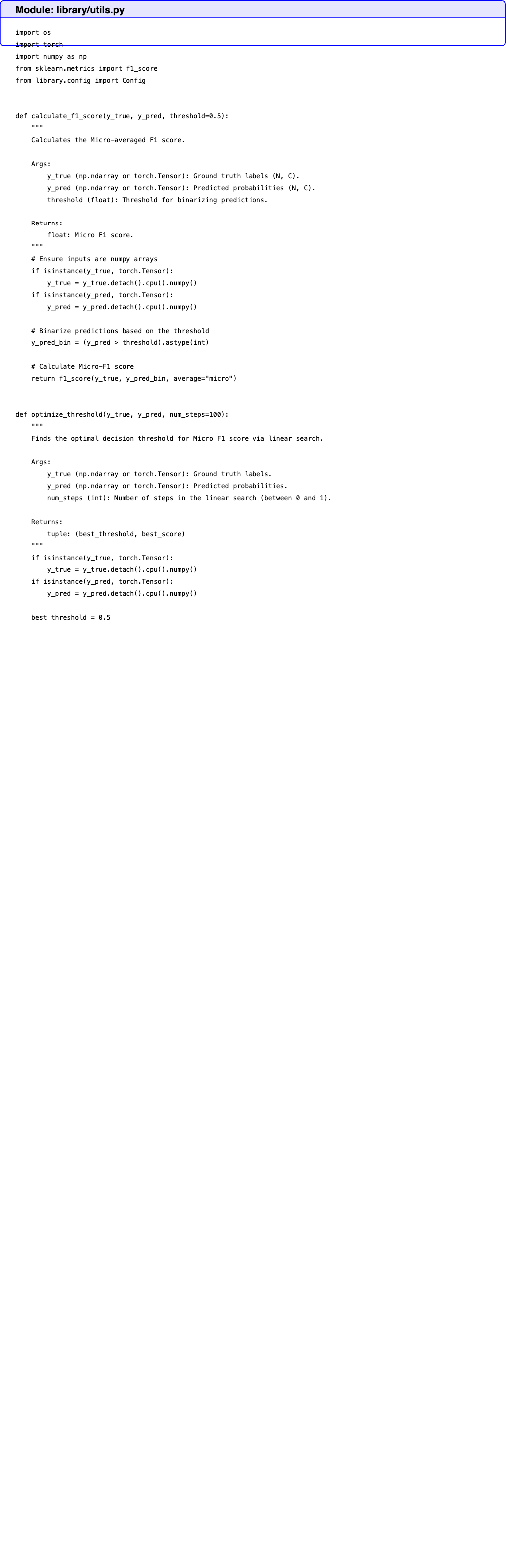
Text in this graphic
Module: library/utils.py
⬇ import os import torch import numpy as np from sklearn.metrics import f1_score from library.config import Config def calculate_f1_score(y_true, y_pred, threshold=0.5): """ Calculates the Micro-averaged F1 score. Args: y_true (np.ndarray or torch.Tensor): Ground truth labels (N, C). y_pred (np.ndarray or torch.Tensor): Predicted probabilities (N, C). threshold (float): Threshold for binarizing predictions. Returns: float: Micro F1 score. """ # Ensure inputs are numpy arrays if isinstance(y_true, torch.Tensor): y_true = y_true.detach().cpu().numpy() if isinstance(y_pred, torch.Tensor): y_pred = y_pred.detach().cpu().numpy() # Binarize predictions based on the threshold y_pred_bin = (y_pred > threshold).astype(int) # Calculate Micro-F1 score return f1_score(y_true, y_pred_bin, average="micro") def optimize_threshold(y_true, y_pred, num_steps=100): """ Finds the optimal decision threshold for Micro F1 score via linear search. Args: y_true (np.ndarray or torch.Tensor): Ground truth labels. y_pred (np.ndarray or torch.Tensor): Predicted probabilities. num_steps (int): Number of steps in the linear search (between 0 and 1). Returns: tuple: (best_threshold, best_score) """ if isinstance(y_true, torch.Tensor): y_true = y_true.detach().cpu().numpy() if isinstance(y_pred, torch.Tensor): y_pred = y_pred.detach().cpu().numpy() best_threshold = 0.5 best_score = -1.0 # Search range from 0.01 to 0.99 to avoid edge cases thresholds = np.linspace(0.01, 0.99, num_steps) for thresh in thresholds: score = calculate_f1_score(y_true, y_pred, threshold=thresh) if score > best_score: best_score = score best_threshold = thresh return best_threshold, best_score def save_checkpoint(model, optimizer, epoch, score, filename): """ Saves a model checkpoint to the working directory. Args: model (torch.nn.Module): The model to save. optimizer (torch.optim.Optimizer): The optimizer state. epoch (int): Current epoch. score (float): Validation score (F1). filename (str): Name of the file to save. """ # Ensure the working directory exists os.makedirs(Config.WORKING_DIR, exist_ok=True) filepath = os.path.join(Config.WORKING_DIR, filename) state = { "epoch": epoch, "model_state_dict": model.state_dict(), "optimizer_state_dict": ( optimizer.state_dict() if optimizer is not None else None ), "score": score, } torch.save(state, filepath) def load_checkpoint(model, filename, optimizer=None, device=Config.DEVICE): """ Loads a model checkpoint. Args: model (torch.nn.Module): The model to load weights into. filename (str): Name of the checkpoint file (relative to WORKING_DIR or absolute). optimizer (torch.optim.Optimizer, optional): Optimizer to load state into. device (str): Device to map location to. Returns: tuple: (epoch, score) """ # Determine full path if os.path.exists(filename): filepath = filename else: filepath = os.path.join(Config.WORKING_DIR, filename) if not os.path.exists(filepath): raise FileNotFoundError(f"Checkpoint file not found: {filepath}") # Load checkpoint checkpoint = torch.load(filepath, map_location=device) # Load model state model.load_state_dict(checkpoint["model_state_dict"]) # Load optimizer state if provided and available if optimizer is not None and checkpoint.get("optimizer_state_dict") is not None: optimizer.load_state_dict(checkpoint["optimizer_state_dict"]) epoch = checkpoint.get("epoch", 0) score = checkpoint.get("score", 0.0) return epoch, score
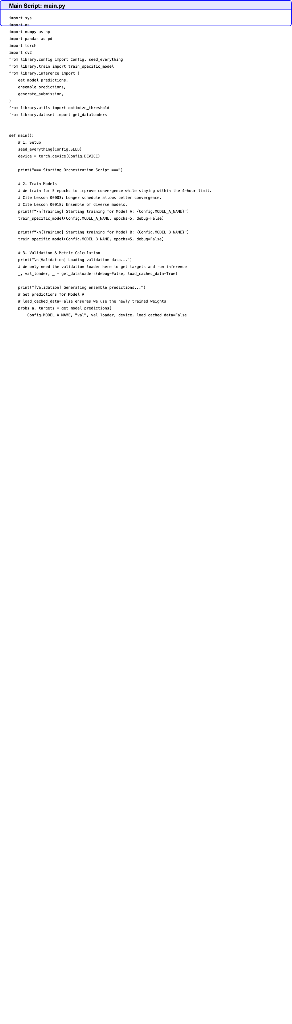
Text in this graphic
Main Script: main.py
⬇ import sys import os import numpy as np import pandas as pd import torch import cv2 from library.config import Config, seed_everything from library.train import train_specific_model from library.inference import ( get_model_predictions, ensemble_predictions, generate_submission, ) from library.utils import optimize_threshold from library.dataset import get_dataloaders def main(): # 1. Setup seed_everything(Config.SEED) device = torch.device(Config.DEVICE) print("=== Starting Orchestration Script ===") # 2. Train Models # We train for 5 epochs to improve convergence while staying within the 4-hour limit. # Cite Lesson 00003: Longer schedule allows better convergence. # Cite Lesson 00018: Ensemble of diverse models. print(f"\n[Training] Starting training for Model A: {Config.MODEL_A_NAME}") train_specific_model(Config.MODEL_A_NAME, epochs=5, debug=False) print(f"\n[Training] Starting training for Model B: {Config.MODEL_B_NAME}") train_specific_model(Config.MODEL_B_NAME, epochs=5, debug=False) # 3. Validation & Metric Calculation print("\n[Validation] Loading validation data...") # We only need the validation loader here to get targets and run inference _, val_loader, _ = get_dataloaders(debug=False, load_cached_data=True) print("[Validation] Generating ensemble predictions...") # Get predictions for Model A # load_cached_data=False ensures we use the newly trained weights probs_a, targets = get_model_predictions( Config.MODEL_A_NAME, "val", val_loader, device, load_cached_data=False ) # Get predictions for Model B probs_b, _ = get_model_predictions( Config.MODEL_B_NAME, "val", val_loader, device, load_cached_data=False ) # Ensemble predictions (simple average) ensemble_probs = ensemble_predictions([probs_a, probs_b]) # Ensure targets are numpy array if isinstance(targets, torch.Tensor): targets = targets.cpu().numpy() elif isinstance(targets, list): targets = np.array(targets) # Optimize threshold best_thresh, best_score = optimize_threshold(targets, ensemble_probs) # REQUIRED OUTPUT print(f"Final Validation Metric: {best_score}") # 4. Failure Analysis print("\n[Analysis] Performing Failure Analysis...") # Calculate per-sample F1 to determine error magnitude # Binarize predictions using the optimal threshold preds_bin = (ensemble_probs > best_thresh).astype(int) # Calculate F1 per sample (instance-level) # F1 = 2*TP / (2*TP + FP + FN) tp = np.sum((preds_bin == 1) & (targets == 1), axis=1) fp = np.sum((preds_bin == 1) & (targets == 0), axis=1) fn = np.sum((preds_bin == 0) & (targets == 1), axis=1) epsilon = 1e-7 f1_samples = (2 * tp) / (2 * tp + fp + fn + epsilon) error_magnitude = 1.0 - f1_samples # Load metadata to get features val_df = pd.read_csv(Config.VAL_CSV) # Feature 1: Label Cardinality (from ground truth) # Handle potential NaNs in attribute_ids val_df["attribute_ids"] = val_df["attribute_ids"].fillna("") val_df["num_labels"] = val_df["attribute_ids"].apply( lambda x: len(x.split()) if x.strip() else 0 ) # Feature 2: Image Brightness (from image content) # We process a subset of validation images to save time sample_size = min(2000, len(val_df)) sample_indices = np.random.choice(len(val_df), size=sample_size, replace=False) brightness_values = [] sampled_errors = [] sampled_cardinality = [] print(f" Processing {sample_size} images for feature extraction...") for idx in sample_indices: row = val_df.iloc[idx] path = os.path.join(Config.INPUT_DIR, row["file_path"]) # Read image img = cv2.imread(path) if img is not None: # Calculate mean brightness b = np.mean(img) / 255.0 brightness_values.append(b) sampled_errors.append(error_magnitude[idx]) sampled_cardinality.append(val_df.iloc[idx]["num_labels"]) # Calculate Correlations if len(sampled_errors) > 1: # Correlation with Label Cardinality corr_card = np.corrcoef(sampled_cardinality, sampled_errors)[0, 1] print(f"Correlation (Error vs Label Cardinality): {corr_card:.4f}") # Correlation with Brightness corr_bright = np.corrcoef(brightness_values, sampled_errors)[0, 1] print(f"Correlation (Error vs Image Brightness): {corr_bright:.4f}") else: print("Insufficient data for correlation analysis.") # 5. Submission THRESHOLD_SCORE = 0.6335639211171432 print(f"\n[Submission] Checking threshold: {best_score} > {THRESHOLD_SCORE}") if best_score > THRESHOLD_SCORE: print("Threshold met. Generating submission file...") # generate_submission handles test inference and saving # load_cached_data=False ensures we generate fresh test predictions generate_submission(debug=False, load_cached_data=False) else: print("Threshold not met. Skipping submission generation.") print("\n=== Workflow Completed ===") if __name__ == "__main__": main()