Direct Pass@ Optimization for Thought Pruning: Balancing Quality and Diversity in Test-Time Reasoning
arXiv:2610.31667v1 · This workspace stays on this version. Check arXiv for newer versions
Some source details need review 5 to check
Original formulas, table values and figures are preserved. Comparison can miss differences; use the original PDF to check details.
Reading view checked: 1199 math expressions, 5 rendering failures; 23 of 23 images available.
Compared 350 of 398 source passages against 41 of 48 PDF pages.
- Some graphics are laid out differently in the HTML source than in the paper (text or formulas outside their frame); check the original PDF. (1)
- Some formulas could not be rendered; their original TeX is shown. Check the original PDF. (5)
- S2_SS0_SSS0_Px3_p3_pic1: the arXiv HTML draws text or formulas of this graphic outside its frame and it could not be corrected safely (too-small); the image shows the HTML layout, which differs from the PDF.
- This long paper was only partially compared; the original sources remain available.
- An unsupported comparison claim was rejected; source verification is incomplete.
23 of 23 figure, table and graphic images captured. Open original PDF
Abstract
Test-time scaling has emerged as a key inference strategy for reasoning models, where a model generates a large number of candidate solutions in the hope of finding at least one correct solution. Running all candidate solutions to completion can be computationally demanding, so recent work prunes the candidate pool after generating only a short prefix, committing further computation only to the surviving candidates. Existing pruning strategies divide broadly into two categories: Quality-based methods assign a score to each partial solution and discard those predicted to ultimately lead to an incorrect final solution, while diversity-based methods select partial solutions that follow different reasoning trajectories and are therefore likely to cover different final solutions. The tension between these two objectives is an instance of exploration versus exploitation, yet little to no prior work on pruning exposes this trade-off directly, let alone optimizes it. In this paper, we introduce a pruning procedure that addresses this trade-off directly by optimizing over the selected solution pool. In particular, it chooses the pool to maximize the probability that at least one of its partial solutions, when continued to completion, yields a correct answer. Because this objective simultaneously rewards high-quality partial solutions and penalizes redundancy among them, quality and diversity are naturally balanced by the criterion itself rather than through separate ad-hoc design choices. On eight open-weight reasoning models, our method outperforms existing quality-based and diversity-based pruning strategies. The gains are particularly pronounced when the pruning procedure keeps a moderate number of partial solutions for continued generation, highlighting the value of directly balancing quality and diversity during pruning.

Large Language Models (LLMs) have demonstrated remarkable capabilities in complex reasoning, showcasing a strong aptitude for solving complex problems that require multi-step logic [45, 21, 52, 18, 15]. To further enhance these capabilities, test-time scaling has emerged as a prominent strategy, where generating multiple candidate solutions for a single problem allows the model to explore diverse reasoning strategies and achieve substantially better final performance [35, 44, 3, 48]. However, a significant challenge in scaling test-time compute is the prohibitive cost of generating many full solutions, which we refer to as rollouts moving forward [33, 23]. Beyond generation, there is also the cost of evaluating the finished rollouts in best-of- methods, which score each rollout with a reward model, and this is computationally demanding on a large pool of long reasoning traces [11, 26, 36]. This computational bottleneck, both in generation and in evaluating all rollouts in best-of- methods, necessitates test-time pruning of partial rollouts before they reach a final answer and terminate. In other words, we generate all rollouts only up to a cutoff of tokens, keep the most promising of them and run those to the full token budget , as illustrated in Fig. 1.
One family of methods examines the confidence dynamics of the model during generation, utilizing metrics such as logit entropy or confidence [30, 50, 17, 43]. The underlying intuition is that if a model is overly confident at an intermediate decoding step, extending the reasoning process is a waste of compute; conversely, if the model is entirely lacking in confidence, it is unlikely to reach a correct solution regardless of the additional compute provided, allowing for early termination. Another line of work leverages the model’s internal state, specifically the hidden states of its transformer blocks, to identify which rollouts are worth continuing [54, 1]. By “probing” these internal states, one can predict whether the model will ultimately arrive at a correct solution, effectively framing the pruning problem as a classification task. This allows for the early discarding of partial rollouts that are unlikely to yield a correct final answer. In parallel, a separate line of research prioritizes representation exploration (RepExp) to select a subset of rollouts that cover as many distinct reasoning strategies as possible [39]. By selecting partial rollouts whose corresponding embeddings are dissimilar, RepExp aims to explore a diverse set of reasoning trajectories.
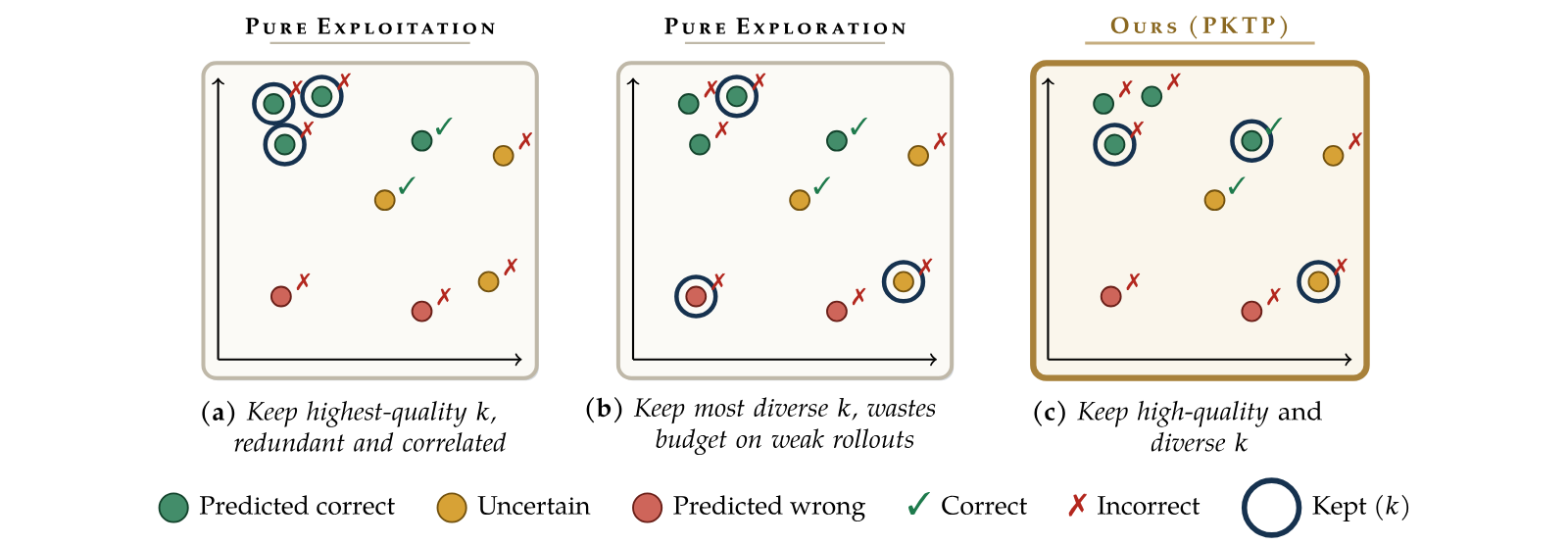
These approaches, however, sit at the two ends of a spectrum, and neither directly optimizes the quantity we actually care about. The problem with probing methods is that the rollouts they rank highest tend to be similar to one another. As a result, the probe may be confidently wrong about all of the kept rollouts at once, and none of them reaches a correct answer. This is the problem of pure exploitation (Fig. 2a). RepExp, on the other hand, finds diverse rollouts, but because it ignores the quality of the rollouts, it can spend much of its budget on rollouts that are unlikely to succeed (Fig. 2b). These limitations motivate selecting the rollouts by the metric we actually want to optimize, choosing the set of rollouts that maximizes , that is, , which we formalize in Eq. 3. Optimizing this objective directly keeps the selected rollouts diverse enough to avoid shared failures while still favoring high-quality ones (Fig. 2c).
To this end, we propose PKTP (Pass@\mathbfit{k} Thought Pruning), a pruning framework that chooses the kept rollouts by maximizing directly. The main difficulty is that, even if the rollouts are sampled independently, their outcomes are not independent (conditioned on the partial observation of the rollout). Hence, depends on their joint distribution (i.e., rollouts with similar partial rollouts tend to succeed or fail together). We model this joint distribution with a latent Gaussian model, in which the correctness of each rollout is obtained by thresholding a Gaussian score. Evaluating under this model requires an expectation over the latent variables, so we instead derive a closed-form second-order approximation of it. We show that this approximation is submodular, enabling us to approximately solve it using a greedy procedure to find a subset of size . An important aspect of the proposed framework is that the latent model is trained only once and does not depend on , and a single greedy pass yields a nested sequence of subsets, so the budget can be chosen online at inference time without retraining.
First, we cast pruning as maximizing the of the kept set, and we model how similar rollouts fail together. Second, we derive a closed-form, submodular approximation of that links the probe and RepExp. Third, through experiments on eight reasoning models, we show that PKTP improves over existing pruning methods, especially for moderate values of .
Given a question \mathbfit{q}, we draw candidate reasoning rollouts y^{(i)}\sim\pi(\,\cdot\mid\mathbfit{q}\,) from a model . Each rollout is observed only through its first tokens, the prefix . We encode this prefix as a representation vector , a hidden-state embedding of the reasoning up to token T. Pruning then keeps rollouts, runs them to the full token budget , and discards the rest. A completed rollout is either correct or not, recorded by the sign ,
Here Verify is a task-specific checker that returns true exactly when a completed rollout reaches a correct final answer, for instance by matching a reference solution on a math problem or passing the unit tests on a coding task. We write for the outcome of the -th rollout once it is run to the budget .
To prune partial rollouts, we need to map each prefix to a vector that captures its essential information. One line of work relies on hand-designed features of the rollout and the model’s internal states, such as token confidence, the geometry of the hidden-state trajectory, or the convergence of intermediate answers. These features are usually very low dimensional [13, 40, 38, 19, 28]. A second line of work instead keeps the hidden states of the transformer and pools them into a single vector [42, 39, 29], and this is the class we use. In particular, we take to be an exponential moving average (EMA) of the hidden states, which has proven an effective pooling operation [29]. Our improvements are thus shown for this class of embeddings, although our framework can be applied to other embeddings as well. Appendix F gives the details of the representation we use.
At pruning time the outcomes are still unknown, since each depends on a (random) continuation we have not yet generated. How, then, should we choose the set of rollouts to keep? Two extreme choices are as follows.
- (i)
(Pure exploitation) Keep in the rollouts with the highest predicted success
\mathbb{P}\!\bigl(C(y^{(i)})=+1\mid\mathbfit{q},y_{1:T}^{(i)}\bigr), estimated by a linear probe trained on the representations [54], that is, the rollouts with the largest scores for a learned weight vector . We refer to this pruning policy as Linear Probe. - (ii)
(Pure exploration) Build a diverse , starting from a random rollout and greedily adding to the rollout by solving
(2)that is, we add, the rollout whose representation is least explained by those already chosen, where is a regularizer. This is the RepExp pruning policy [39].
Neither extreme balances quality against diversity. What we actually want is the set of rollouts with the best . Mathematically, we seek the set most likely to contain a correct rollout,

Text in this graphic
Pass@ Pruning Objective
\max_{S\,\subseteq\,\{1,\ldots,N\}}\mathbb{P}\!\left(\,\sum_{i\in S}\mathbf{1}\{C(y^{(i)})=+1\}\;\geq\;1\;\middle|\;\mathbfit{q},\,y_{1:T}^{(1)},\ldots,y_{1:T}^{(N)}\,\right)\quad\text{s.t.}\quad|S|=k.Here, is the indicator function, i.e., and . The objective in Eq. 3 is exactly of the kept pool, the probability that at least one surviving rollout, once run to the budget , yields a correct answer. We also assume that the final outcomes are binary, although the same approach generalizes to continuous outcomes, where each completed rollout is scored by a reward model and the goal is to maximize the best of the kept rollouts [10], in which case Eq. 3 becomes a max@ objective [41].
Existing pruning methods score each rollout on its own, using the model’s confidence [30, 13], a reward model [36], or a probe on its hidden states [54, 25], or they select a diverse set, as RepExp does [39]. Pass@ has also been used as a training objective for reasoning models [41, 8], but not to decide which partial rollouts to keep. Outside of language models, choosing a set so that at least one item succeeds has been studied in information retrieval and Bayesian optimization [6, 34, 46]. Appendix G gives an extended discussion. In what follows, we discuss how such an objective can be solved.
There are some challenges in solving Eq. 3: First, we need to obtain the of a given set of rollouts. We address this by learning the joint distribution of the rollouts’ outcomes under a probabilistic model, from which the of any set can be estimated. Second, even with such an estimate, finding the subset of rollouts with the highest estimated is a mixed-integer program. We can therefore view our framework as two components, learning the joint distribution of the outcomes (Section 3.1), and solving this mixed-integer program at selection time (Section 3.2).
Let collect the representations of the generated partial rollouts, be a learnable mapping predicting the rollout quality, and define with . We model the latent scores of the rollouts as
where and are independent. Intuitively, is a score of how promising rollout is, so the higher its quality , the higher its score. On top of , the term is a random effect shared by rollouts with similar representations, which makes them succeed or fail together. Indeed, for distinct rollouts, , so rollouts with aligned have positively correlated outcomes. Finally, is noise specific to rollout .
The correctness of rollout is then modeled by thresholding its score at zero. More specifically, we define the random variable . In other words, a positive score implies that the rollout is correct, while a negative score implies that it is incorrect. Since the scores are independent conditionally on , the likelihood of an observed correctness pattern is
where is the standard Gaussian CDF, and the derivation can be found in Section A.1.
Suppose we have training questions, where question consists of the representations of a pool and its observed outcomes . The mapping is trained by maximizing their likelihood under Eq. 5, that is, by solving
where is the likelihood of Eq. 5 with and . Solving Eq. 6 directly is hard, since the expectation over in Eq. 5 has no closed form. We therefore expand each log-factor to second order in , which turns the expectation into a Gaussian integral that can be evaluated exactly (Theorem 1).
For a pattern , let be the standard Gaussian density, , ,
Then, as ,
and replacing each log-factor of in Eq. 5 by this expansion at gives
The proof is in Section B.1.1. The expansion is local, so we use Eq. 9 as a tractable surrogate rather than as an exact identity or a bound. We therefore replace in Eq. 6 by .
Instead of using directly in the correlation term, one could learn an encoder of the representations and use in its place, but its helpfulness depends on the amount of data. Since our data is limited, we keep fixed, so that is the only learned component, and for the same reason we use a simple linear model for , as in the Linear Probe [54]. Unlike the Linear Probe, which is trained on the correctness of each rollout separately, is trained on the joint outcomes of all rollouts of a question, so the quality it learns already accounts for the correlation between them. Since Eq. 9 is in closed form and differentiable in , we maximize the surrogate likelihood by stochastic gradient ascent over the training questions.
Maximizing in Eq. 3 is the same as minimizing the probability that every kept rollout fails. Under the latent Gaussian model, and suppressing the conditioning on , the failure probability of a set of kept rollouts is
and we seek the set of rollouts that minimizes it. Since has no closed form, we approximate it with Theorem 1.
For a set , let , , and . Applying Theorem 1 to the rollouts in with for every gives a surrogate of with
The proof is in Section B.1.2. We therefore minimize over . Each term of Eq. 11 has a direct interpretation. The first term favors large , because the baseline failure factor decreases with . The negative log-determinant rewards a collection of ’s that covers several directions instead of repeatedly selecting the same direction. The last term is nonnegative and penalizes sets whose weighted vectors add up in the same direction, which the determinant alone cannot detect since it treats and identically. For example, two rollouts of the same quality fail together more often with than with , yet both cases give the same and hence the same determinant, while is in the first case and in the second.
However, minimizing exactly is hard.
Minimizing over all with is NP-hard.
The proof is in Section B.3, by a reduction from the maximum independent set problem. When the objective is monotone and submodular, however, a greedy optimizer that adds one rollout at a time is guaranteed to achieve at least a fraction of the optimal value [32]. The exact pass probability is known to be monotone and submodular [46]. An approximation of a submodular function, though, is not necessarily submodular, so we prove that its surrogate is also monotone and submodular, and hence the greedy optimizer and its approximation guarantee apply to our problem.
is normalized (), monotone ( whenever ), and submodular, that is, for all and ,
Consequently, the set obtained by adding, times, the candidate that most increases satisfies
The proof is in Section B.2.
The greedy optimizer starts from the empty set and, at each step, adds the candidate with the smallest change . Since adding a candidate changes by a rank-one matrix, this change has a closed form that can be updated cheaply without rebuilding the determinant and the inverse (Section A.2). With these rank-one updates, the greedy optimizer costs time and memory. By comparison, a naive implementation that rebuilds and factorizes for every candidate costs per candidate, that is, time, with the same memory.
The surrogate makes the quality–diversity trade-off explicit and connects to the two baseline criteria in limiting regimes. If the correlation term in Eq. 11 is switched off, then , so minimizing it keeps the largest quality scores and recovers a quality-only, probe-style ranking; it coincides with Linear Probe when is the corresponding linear probe. At the other extreme, suppose that the quality scores are equal and that the penalty term is negligible throughout selection. Then every equals a common value , so and the relevant set-dependent term is . By the matrix determinant lemma, its greedy marginal ranks a candidate by , the residual-variance criterion used by RepExp on the same representations (see Section A.3 for the derivation). Between these limits, the modular quality, log-determinant diversity, and penalty terms jointly determine the selected set.
The above two extremes do not show how PKTP moves from Linear Probe to RepExp as grows. To see this, we expand and its surrogate when the correlations are weak.
Fix , and , and replace by . As ,
and has the same expansion.
Proposition 2 shows how the correlation strength controls where PKTP sits between the two baselines. At the rollouts are independent, the expansion reduces to , and PKTP ranks the rollouts by quality, as Linear Probe does. For , every pair of kept rollouts adds a penalty , which is large when their representations are similar. A rollout added to a set of rollouts pays such penalties, so the first pick is decided by quality alone, and as the set grows the penalties add up until they outweigh the differences in quality, after which PKTP spreads its picks out, as RepExp does. The larger is, the sooner this happens, so sets how fast PKTP moves from Linear Probe to RepExp as grows.
Appendix C makes the two ends of this behavior precise for a fixed . At small , if the gap between the th and th largest qualities exceeds a constant multiple of , PKTP keeps exactly the candidates with the largest , as Linear Probe does, and in the same order when this holds at every budget up to . At large , when a few candidates of high quality stand out from a bulk of lower quality, the objective of PKTP, averaged over the bulk qualities, reduces to the RepExp objective plus a term for these candidates. Its minimizers therefore keep them and nearly maximize the RepExp objective. Finally, the conditions of these two results do not conflict. We construct a single model, with one quality distribution and one value of , in which PKTP follows Linear Probe at small , while its averaged objective reduces to the RepExp objective as grows.
We evaluate on eight open-weight reasoning models in two size tiers. The small tier is Qwen3-0.6B, Qwen3-1.7B [49], OpenMath-Nemotron-1.5B [31] and DeepSeek-R1-Distill-Qwen-1.5B [15], and the large tier is Qwen3-8B, OpenMath-Nemotron-7B, DeepSeek-R1-Distill-Qwen-7B and Skywork-OR1-Math-7B [16]. Every model generates its rollouts with temperature , top- of , and a full token budget of tokens.
We pool problems from several benchmark sources rather than a single one, since a pruning policy has to be trained on part of the problems and evaluated on the rest, and no single competition benchmark is large enough for both. The two model tiers are evaluated on different benchmark substrates, chosen so that neither tier is saturated. Both tiers use AIME 2024, 2025 and 2026 and HMMT 2024, 2025 and 2026 [2], together with RIMO-N [9]. The small tier adds BeyondAIME [4], OlymMATH (Easy) [37] and Omni-MATH levels 7 and 8 [14], while the large tier replaces these by AMO-Bench [27], OlymMATH (Hard) and Omni-MATH levels 8 and 9. This gives around problems per model. For each model we then remove the problems on which it generates all correct or all wrong solutions in trials.
A completed rollout counts as correct when its final answer matches the reference answer of the problem. We take that answer from the \boxed{} expression of the rollout and ask a Qwen3-32B judge [49] whether it is equivalent to the reference answer. We use a judge rather than a symbolic checker such as math-verify [24], because benchmarks like AMO-Bench have descriptive answers that a symbolic checker cannot handle.
Only a few hundred problems are available for each model, so a single split into training and test problems would leave too few on either side, and we evaluate with cross-validation instead. For each model we partition its problems into eight folds, with each benchmark spread evenly across the folds. Each fold serves once as the test set while the learned components are trained on the other seven, so every problem is scored exactly once by a model that was not trained on it. One such pass over all eight folds forms a repetition. Because the outcome of a repetition depends on how the problems happen to be divided, we run repetitions, each with a new random partition obtained by shuffling the problems of every benchmark before assigning them to folds, and with fresh random seeds for training. Every reported number is the average over the repetitions, and its standard error is computed across them. For RepExp we set the regularizer to . For all methods, the representation of a partial rollout is the EMA of its hidden states with rate .
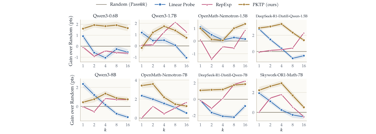
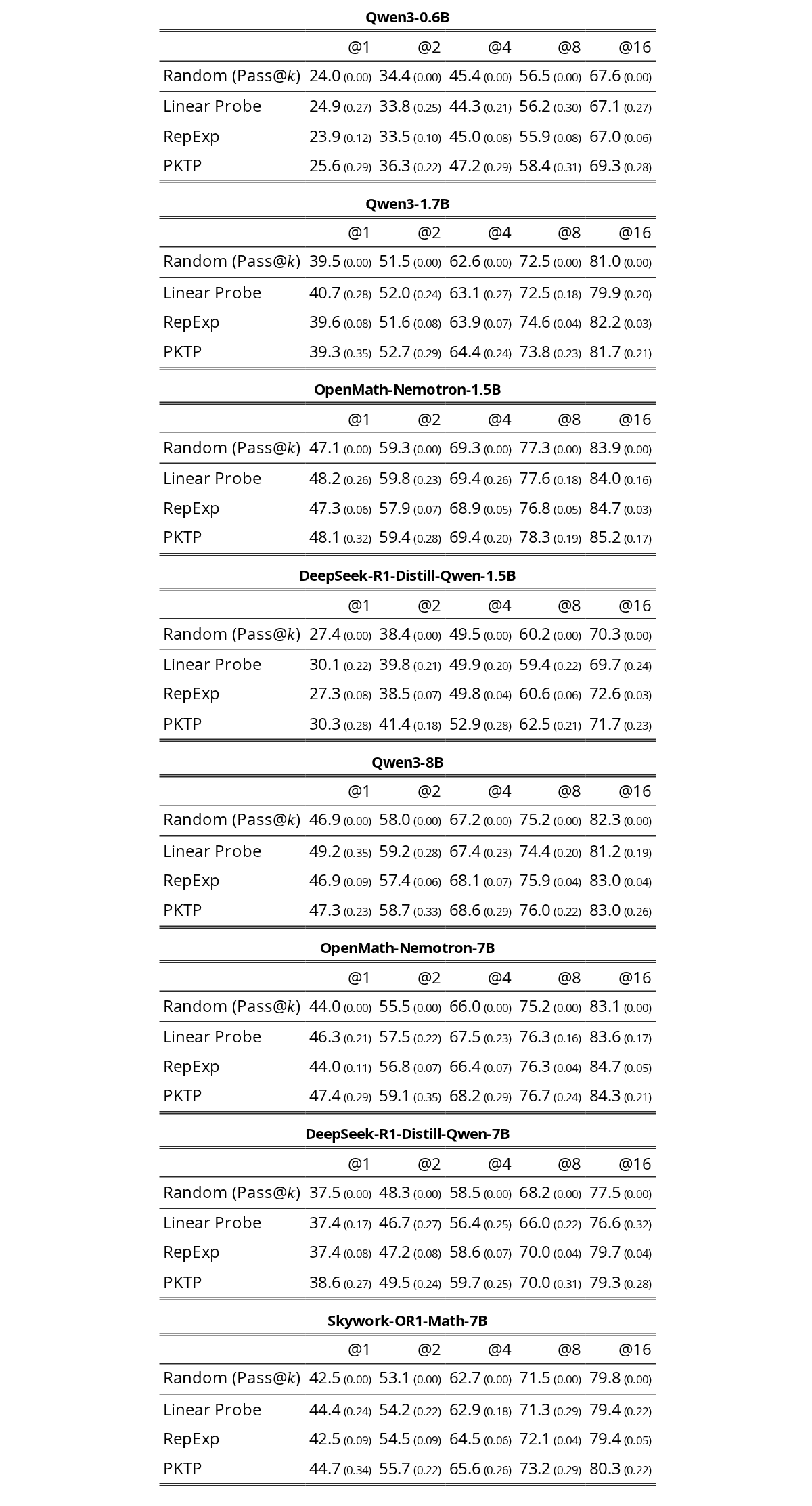
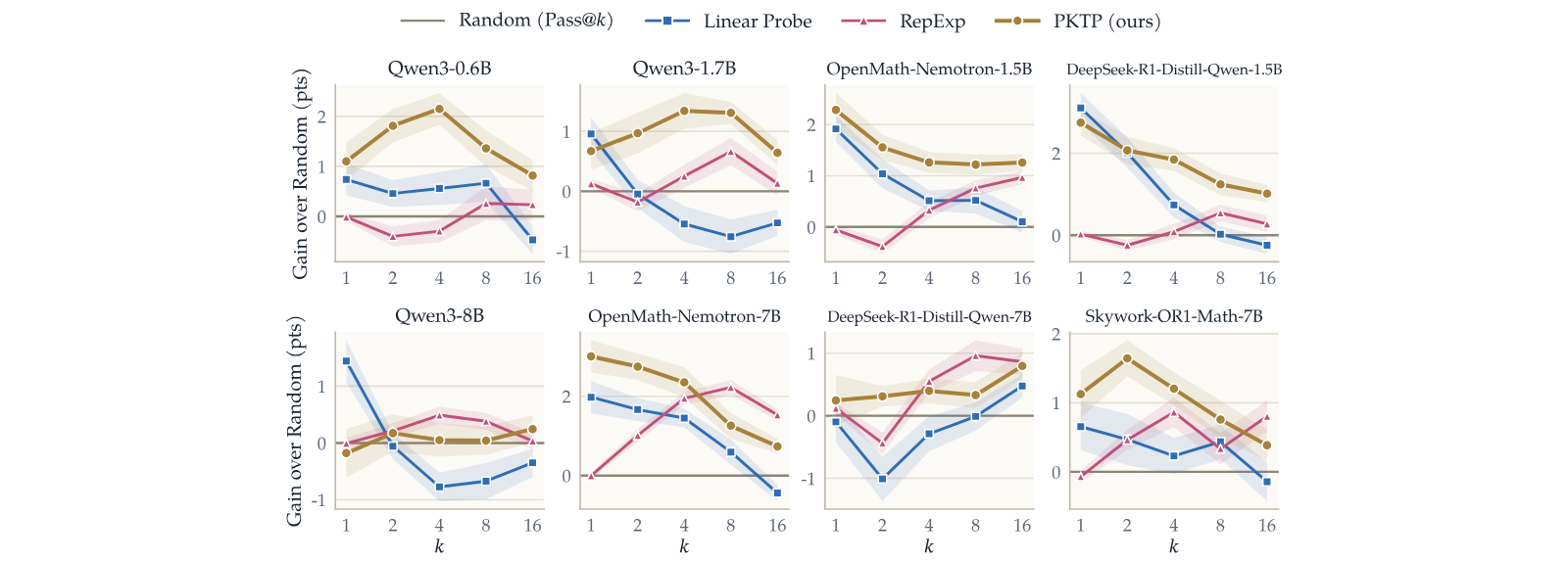
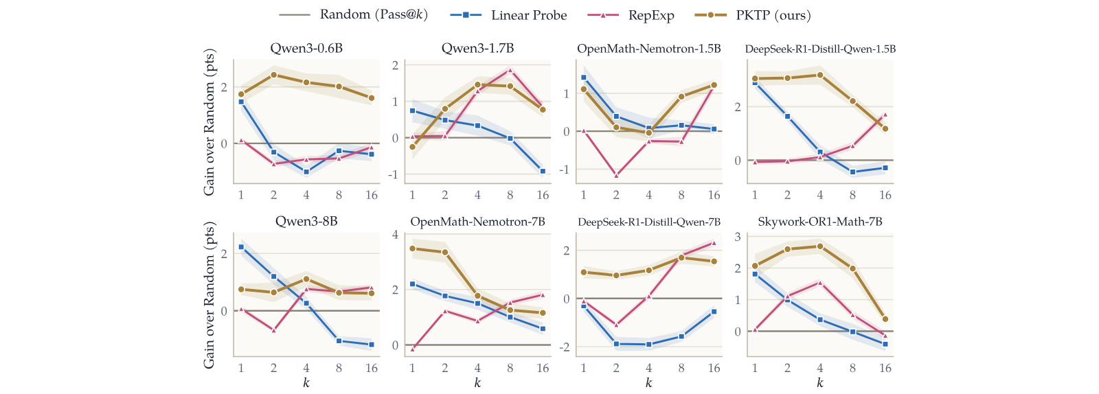
Figure 3 reports our main setting, in which each method selects of the rollouts of a problem from their prefixes, and we set the cutoff threshold to tokens. For every model it shows the of each pruning policy minus that of Random (Pass@), pooled over all test problems. Random keeps rollouts chosen uniformly at random, which is equivalent to sampling rollouts without any pruning, so it is the natural reference point. The absolute numbers are given in Table 1 and the breakdown by benchmark in Appendix D.

As evident in Fig. 3, the Linear Probe performs strongly at , but as increases it gets closer and closer to Random, as in the Qwen models, and in some cases it even becomes worse than Random at large . This can be attributed to a bias towards a cluster of rollouts that the model predicts to be correct but that may not be, in the case where the classifier is wrong. In other words, ranking by the probe sharpens the distribution of the kept rollouts around what the probe considers correct. This mirrors the effect observed in reinforcement learning, where models trained with GRPO outperform their base models at small but are outperformed by them at large [53]. As an example, Fig. 4 shows the rollouts of one problem (Qwen3-8B, AMO-Bench), projected on the first two principal components of their representations. The rollouts ranked highest by the probe are all close to each other and all wrong, while random picks include correct ones.

Figure 3 also shows that RepExp behaves in the opposite way to the Linear Probe. At it shows, as expected, a performance similar to Random, since its first pick is random. As increases, the general trend is that RepExp gets better and better than Random, especially at (e.g., the DeepSeek-R1-Distill models). Interestingly, however, for moderate it is sometimes outperformed by Random, for instance on OpenMath-Nemotron-1.5B and Qwen3-8B. We attribute this to a tendency of RepExp to favor outliers at small and moderate , since the rollouts farthest from those already selected are often unusual rollouts that are unlikely to be correct. A similar effect is reported by Tuyls et al. 39, where RepExp stops helping under high-temperature sampling, since the less coherent responses look novel in representation space yet do not necessarily contain correct answers. As an example, Fig. 5 shows the rollouts of one problem (Qwen3-8B, Omni-MATH), embedded in two dimensions with multidimensional scaling on their representations. After its first, random pick, RepExp selects outliers far from the other rollouts, and all of its picks are wrong, while random picks include correct one.
Finally, Fig. 3 shows that PKTP outperforms both the Linear Probe and RepExp, and its advantage is clearest at moderate , where each baseline suffers from its own bias. On DeepSeek-R1-Distill-Qwen-1.5B at , for example, PKTP is points above the Linear Probe and points above RepExp. On Qwen3-0.6B it leads both baselines by more than points at every , and on DeepSeek-R1-Distill-Qwen-7B it is points above the Linear Probe at . Unlike the two baselines, PKTP also stays above Random on every model for , since it keeps the correctness signal of the probe while spreading the kept rollouts over outcomes that are unlikely to fail together. At large , however, the performance of PKTP and RepExp gets closer. We believe this is due to the weak correctness signal in the embeddings of the partial rollouts, which raises the question of how a quality embedding can be obtained from a partial rollout, and whether this is possible at all.
Results for the other pool sizes, with the same cutoff , are given in Appendix E.

An important aspect of pruning is the cutoff threshold , and how the algorithm behaves as the cutoff grows. Figure 6 varies on Qwen3-1.7B and DeepSeek-R1-Distill-Qwen-7B. For every , PKTP outperforms all other methods on both models. An interesting observation is that a later cutoff in general improves the performance of PKTP. On Qwen3-1.7B its pass@ rises from at to at , and on DeepSeek-R1-Distill-Qwen-7B from to . Intuitively, the more tokens are generated, the more is revealed about the quality of a rollout and where it is heading, so there is more signal to exploit. Interestingly, however, the same does not necessarily happen for the Linear Probe and RepExp. On Qwen3-1.7B, for example, the Linear Probe drifts down from to and ends below Random. One reason can be the representation we use. Since the EMA with rate effectively averages over the last tokens, it may lose the signal in the earlier tokens.

Another important aspect of pruning is the size of the pool the rollouts are chosen from. Figure 7 varies on Qwen3-1.7B and DeepSeek-R1-Distill-Qwen-7B. PKTP outperforms all other methods for every on Qwen3-1.7B, and on DeepSeek-R1-Distill-Qwen-7B once the pool reaches . A larger pool offers more candidates to choose from, and on Qwen3-1.7B both baselines benefit from it, with RepExp rising from at to at as the pool becomes more diverse and the Linear Probe from to . Interestingly, however, the same does not hold on DeepSeek-R1-Distill-Qwen-7B, where the Linear Probe falls from to and stays below Random for every , and RepExp falls from at to , while PKTP rises from to . One reason can be that a larger pool also contains more outliers, which raises the chance that extreme cases like RepExp and the Linear Probe select them at a moderate such as .
We introduced PKTP, a pruning framework that chooses which partial rollouts to keep by directly optimizing . PKTP learns the joint distribution of the rollouts’ outcomes with a latent Gaussian model, approximates the resulting likelihood in closed form, and selects the kept set greedily, with an approximation guarantee on the surrogate objective. Across eight reasoning models, it outperforms both quality-based and diversity-based pruning, and the gains are largest at moderate , where each of these baselines suffers from its own bias. Since PKTP can be combined with any representation of partial rollouts, representations that better capture the correctness of a rollout would directly strengthen it, and developing them is a natural direction for future work.
This work was supported in part by a Generative AI Research Award from the USC Office of Research and Innovation, the NSF NRT program, the USC-Meta Center for Research and Education in AI and Learning, and a gift from Amazon. AJ was supported in part by the NSF Award DMS-2311024, an Amazon Faculty Research Award, an Adobe Faculty Research Award, and an iORB grant from USC Marshall School of Business.
In this work, we used generative AI tools to assist with several parts of the project. For the write-up, we used them to edit and polish the text and to format the LaTeX source. For the figures, we used them to write the scripts that plot our experimental results. For the code, we used them to help implement parts of our implementation. For the theory, we used them to help derive and write parts of the proofs in the appendix. We have not used generative AI tools to generate data or experimental results. All AI-assisted content, including the code and the proofs, was reviewed and verified by the authors, who take full responsibility for the content of this paper.
References
- [1] A. Afzal, F. Matthes, G. Chechik, and Y. Ziser (2025) Knowing before saying: LLM representations encode information about chain-of-thought success before completion. In Findings of the Association for Computational Linguistics: ACL 2025, pp. 12791–12806. Cited by: Appendix G, §1.
- [2] M. Balunović, J. Dekoninck, I. Petrov, N. Jovanović, and M. Vechev (2025) MathArena: evaluating LLMs on uncontaminated math competitions. In Advances in Neural Information Processing Systems, Datasets and Benchmarks Track, Cited by: §4.1.
- [3] B. Brown, J. Juravsky, R. Ehrlich, R. Clark, Q. V. Le, C. Ré, and A. Mirhoseini (2024) Large language monkeys: scaling inference compute with repeated sampling. arXiv preprint arXiv:2407.21787. Cited by: Appendix G, §1.
- [4] ByteDance Seed (2025) Seed1.5-Thinking: advancing superb reasoning models with reinforcement learning. arXiv preprint arXiv:2504.13914. Cited by: §4.1.
- [5] J. Carbonell and J. Goldstein (1998) The use of MMR, diversity-based reranking for reordering documents and producing summaries. In Proceedings of the 21st Annual International ACM SIGIR Conference on Research and Development in Information Retrieval, Cited by: Appendix G.
- [6] H. Chen and D. R. Karger (2006) Less is more: probabilistic models for retrieving fewer relevant documents. In Proceedings of the 29th Annual International ACM SIGIR Conference on Research and Development in Information Retrieval, pp. 429–436. Cited by: Appendix G, §2.
- [7] Y. Chen, S. Chakraborty, L. Wolf, Y. Paschalidis, and A. Pacchiano (2026) Post-training large language models for diverse high-quality responses. In International Conference on Learning Representations, Cited by: Appendix G.
- [8] Z. Chen, X. Qin, Y. Wu, Y. Ling, Q. Ye, W. X. Zhao, and G. Shi (2025) Pass@k training for adaptively balancing exploration and exploitation of large reasoning models. arXiv preprint arXiv:2508.10751. Cited by: Appendix G, §2.
- [9] Z. Chen, C. Qin, and Y. Shu (2025) RIMO: an easy-to-evaluate, hard-to-solve olympiad benchmark for advanced mathematical reasoning. arXiv preprint arXiv:2509.07711. Cited by: §4.1.
- [10] Y. Chow, G. Tennenholtz, I. Gur, V. Zhuang, B. Dai, S. Thiagarajan, C. Boutilier, R. Agarwal, A. Kumar, and A. Faust (2025) Inference-aware fine-tuning for best-of-N sampling in large language models. In International Conference on Learning Representations, Cited by: Appendix G, §2.
- [11] K. Cobbe, V. Kosaraju, M. Bavarian, M. Chen, H. Jun, L. Kaiser, M. Plappert, J. Tworek, J. Hilton, R. Nakano, C. Hesse, and J. Schulman (2021) Training verifiers to solve math word problems. arXiv preprint arXiv:2110.14168. Cited by: §1.
- [12] R. Durrett (2019) Probability: theory and examples. 5th edition, Cambridge University Press. External Links: Document Cited by: §B.2.2, §B.2.2.Source
- [13] Y. Fu, X. Wang, H. Zhang, Y. Tian, and J. Zhao (2026) Deep think with confidence. In International Conference on Learning Representations, Cited by: Appendix G, §2, §2.
- [14] B. Gao, F. Song, Z. Yang, Z. Cai, Y. Miao, Q. Dong, L. Li, C. Ma, L. Chen, R. Xu, et al. (2025) Omni-MATH: a universal olympiad level mathematic benchmark for large language models. In International Conference on Learning Representations, Cited by: §4.1.
- [15] D. Guo, D. Yang, H. Zhang, J. Song, P. Wang, Q. Zhu, R. Xu, R. Zhang, S. Ma, X. Bi, et al. (2025) DeepSeek-R1 incentivizes reasoning in LLMs through reinforcement learning. Nature 645 (8081), pp. 633–638. Cited by: §1, §4.1.
- [16] J. He, J. Liu, C. Y. Liu, R. Yan, C. Wang, P. Cheng, X. Zhang, F. Zhang, J. Xu, W. Shen, et al. (2025) Skywork open reasoner 1 technical report. arXiv preprint arXiv:2505.22312. Cited by: §4.1.
- [17] P. Hosseini, S. Nawathe, M. Salmani, M. Razaviyayn, and S. Feizi (2026) Early stopping for large reasoning models via confidence dynamics. arXiv preprint arXiv:2604.04930. Cited by: §1.
- [18] A. Jaech, A. Kalai, A. Lerer, A. Richardson, A. El-Kishky, A. Low, A. Helyar, A. Madry, A. Beutel, A. Carney, et al. (2024) OpenAI o1 system card. arXiv preprint arXiv:2412.16720. Cited by: §1.
- [19] X. Jiang, N. Liu, D. Wang, and L. Hu (2026) Beyond scalars: evaluating and understanding LLM reasoning via geometric progress and stability. In International Conference on Machine Learning, Cited by: §2.
- [20] R. M. Karp (1972) Reducibility among combinatorial problems. In Complexity of Computer Computations, pp. 85–103. Cited by: §B.3.
- [21] T. Kojima, S. S. Gu, M. Reid, Y. Matsuo, and Y. Iwasawa (2022) Large language models are zero-shot reasoners. Advances in Neural Information Processing Systems 35, pp. 22199–22213. Cited by: §1.
- [22] A. Kulesza and B. Taskar (2012) Determinantal point processes for machine learning. Foundations and Trends in Machine Learning 5 (2–3), pp. 123–286. Cited by: Appendix G.
- [23] W. Kwon, Z. Li, S. Zhuang, Y. Sheng, L. Zheng, C. H. Yu, J. Gonzalez, H. Zhang, and I. Stoica (2023) Efficient memory management for large language model serving with PagedAttention. In Proceedings of the 29th Symposium on Operating Systems Principles, pp. 611–626. Cited by: §1.
- [24] H. Kydlíček (2025) Math-Verify: math verification library. Note: https://github.com/huggingface/Math-Verify Cited by: §4.1.Source
- [25] Z. Liang, B. Huang, Z. Wang, and M. Zhang (2026) Hidden states as early signals: step-level trace evaluation and pruning for efficient test-time scaling. In Findings of the Association for Computational Linguistics: ACL 2026, pp. 26800–26813. Cited by: Appendix G, §2.
- [26] H. Lightman, V. Kosaraju, Y. Burda, H. Edwards, B. Baker, T. Lee, J. Leike, J. Schulman, I. Sutskever, and K. Cobbe (2024) Let’s verify step by step. In International Conference on Learning Representations, Cited by: §1.
- [27] J. Liu, S. An, S. Zhou, D. Ma, Y. Lin, X. Lv, X. Wang, X. Li, Z. Wang, X. Cao, and X. Cai (2026) AMO-Bench: large language models still struggle in high school math competitions. In Findings of the Association for Computational Linguistics: ACL 2026, pp. 2120–2137. Cited by: §4.1.
- [28] X. Liu and L. Wang (2025) Answer convergence as a signal for early stopping in reasoning. In Proceedings of the 2025 Conference on Empirical Methods in Natural Language Processing, pp. 17896–17907. Cited by: §2.
- [29] H. Lu, M. Pan, R. Li, G. Nan, J. Zhuang, Z. Zhao, Z. Sun, K. Wang, and Y. Liu (2026) Streaming hallucination detection in long chain-of-thought reasoning. In Findings of the Association for Computational Linguistics: ACL 2026, pp. 21157–21183. Cited by: §2.
- [30] R. Manvi, A. Singh, and S. Ermon (2024) Adaptive inference-time compute: LLMs can predict if they can do better, even mid-generation. arXiv preprint arXiv:2410.02725. Cited by: Appendix G, §1, §2.
- [31] I. Moshkov, D. Hanley, I. Sorokin, S. Toshniwal, C. Henkel, B. Schifferer, W. Du, and I. Gitman (2025) AIMO-2 winning solution: building state-of-the-art mathematical reasoning models with OpenMathReasoning dataset. arXiv preprint arXiv:2504.16891. Cited by: §4.1.
- [32] G. L. Nemhauser, L. A. Wolsey, and M. L. Fisher (1978) An analysis of approximations for maximizing submodular set functions. Mathematical Programming 14 (1), pp. 265–294. Cited by: §B.2.3, Appendix G, §3.2.
- [33] R. Pope, S. Douglas, A. Chowdhery, J. Devlin, J. Bradbury, J. Heek, K. Xiao, S. Agrawal, and J. Dean (2023) Efficiently scaling transformer inference. Proceedings of Machine Learning and Systems 5, pp. 606–624. Cited by: §1.
- [34] S. Sanner, S. Guo, T. Graepel, S. Kharazmi, and S. Karimi (2011) Diverse retrieval via greedy optimization of expected 1-call@k in a latent subtopic relevance model. In Proceedings of the 20th ACM International Conference on Information and Knowledge Management, Cited by: Appendix G, §2.
- [35] C. Snell, J. Lee, K. Xu, and A. Kumar (2025) Scaling LLM test-time compute optimally can be more effective than scaling parameters for reasoning. In International Conference on Learning Representations, Cited by: Appendix G, §1.
- [36] H. Sun, M. Haider, R. Zhang, H. Yang, J. Qiu, M. Yin, M. Wang, P. Bartlett, and A. Zanette (2024) Fast best-of-N decoding via speculative rejection. In Advances in Neural Information Processing Systems, Cited by: Appendix G, §1, §2.
- [37] H. Sun, Y. Min, Z. Chen, W. X. Zhao, and J. Wen (2026) Challenging the boundaries of reasoning: an olympiad-level math benchmark for large language models. In Proceedings of the 64th Annual Meeting of the Association for Computational Linguistics (Volume 1: Long Papers), pp. 17438–17457. Cited by: §4.1.
- [38] L. Sun, H. Dong, B. Qiao, Q. Lin, D. Zhang, and S. Rajmohan (2026) LLM reasoning as trajectories: step-specific representation geometry and correctness signals. In Proceedings of the 64th Annual Meeting of the Association for Computational Linguistics (Volume 1: Long Papers), pp. 26872–26887. Cited by: §2.
- [39] J. Tuyls, D. J. Foster, A. Krishnamurthy, and J. T. Ash (2026) Representation-based exploration for language models: from test-time to post-training. In International Conference on Learning Representations, Cited by: Appendix G, §1, item (ii), §2, §2, §4.2.
- [40] M. G. Vilas, S. Yousefi, B. Nushi, E. Horvitz, and V. Balachandran (2026) Tracing the traces: latent temporal signals for efficient and accurate reasoning. In International Conference on Learning Representations, Cited by: §2.
- [41] C. Walder and D. T. Karkhanis (2025) Pass@K policy optimization: solving harder reinforcement learning problems. In Advances in Neural Information Processing Systems, Vol. 38, pp. 152416–152445. Cited by: Appendix G, §2, §2.
- [42] S. L. Wang, P. Isola, and B. Cheung (2026) The truth lies somewhere in the middle (of the generated tokens). In International Conference on Machine Learning, Cited by: §2.
- [43] X. Wang, J. McInerney, L. Wang, and N. Kallus (2025) Entropy after </think> for reasoning model early exiting. arXiv preprint arXiv:2509.26522. Cited by: §1.
- [44] X. Wang, J. Wei, D. Schuurmans, Q. Le, E. Chi, S. Narang, A. Chowdhery, and D. Zhou (2023) Self-consistency improves chain of thought reasoning in language models. In International Conference on Learning Representations, Cited by: Appendix G, §1.
- [45] J. Wei, X. Wang, D. Schuurmans, M. Bosma, B. Ichter, F. Xia, E. Chi, Q. V. Le, and D. Zhou (2022) Chain-of-thought prompting elicits reasoning in large language models. Advances in Neural Information Processing Systems 35, pp. 24824–24837. Cited by: §1.
- [46] J. T. Wilson, F. Hutter, and M. P. Deisenroth (2018) Maximizing acquisition functions for Bayesian optimization. In Advances in Neural Information Processing Systems, Cited by: §B.2, Appendix G, §2, §3.2.
- [47] X. Wu, L. Bai, H. Bansal, P. Kung, S. Li, H. Liu, N. Peng, and K. Chang (2026) Planned test-time scaling with coordinated reasoning paths. arXiv preprint arXiv:2609.27374. Cited by: Appendix G.
- [48] Y. Wu, Z. Sun, S. Li, S. Welleck, and Y. Yang (2025) Inference scaling laws: an empirical analysis of compute-optimal inference for LLM problem-solving. In International Conference on Learning Representations, Cited by: Appendix G, §1.
- [49] A. Yang, A. Li, B. Yang, B. Zhang, B. Hui, B. Zheng, B. Yu, C. Gao, C. Huang, C. Lv, et al. (2025) Qwen3 technical report. arXiv preprint arXiv:2505.09388. Cited by: §4.1, §4.1.
- [50] C. Yang, Q. Si, Y. Duan, Z. Zhu, C. Zhu, Q. Li, M. Chen, Z. Lin, and W. Wang (2026) Dynamic early exit in reasoning models. In International Conference on Learning Representations, Vol. 2026, pp. 88170–88210. Cited by: §1.
- [51] L. Yang, H. Luo, J. Zhao, T. Dao, and R. Netravali (2026) Thought-level beam search for reasoning. In Conference on Language Modeling, Cited by: Appendix G.
- [52] S. Yao, D. Yu, J. Zhao, I. Shafran, T. Griffiths, Y. Cao, and K. Narasimhan (2023) Tree of thoughts: deliberate problem solving with large language models. Advances in Neural Information Processing Systems 36, pp. 11809–11822. Cited by: §1.
- [53] Y. Yue, Z. Chen, R. Lu, A. Zhao, Z. Wang, Y. Yue, S. Song, and G. Huang (2025) Does reinforcement learning really incentivize reasoning capacity in LLMs beyond the base model?. In Advances in Neural Information Processing Systems, Cited by: §4.2.
- [54] A. Zhang, Y. Chen, J. Pan, C. Zhao, A. Panda, J. Li, and H. He (2025) Reasoning models know when they’re right: probing hidden states for self-verification. In Conference on Language Modeling, Cited by: Appendix G, §1, item (i), §2, §3.1.
Write . Conditioned on , the are independent of each other, so
Since the standard Gaussian is symmetric about , follows the same distribution as , and with each factor equals . Taking the expectation with respect to on both sides gives Eq. 5.
As in Corollary 1, let and . Write , and . Adding a candidate changes by the rank-one matrix . The matrix determinant lemma gives
while Sherman–Morrison gives
Substituting Eq. 18 and Eq. 19 into Eq. 11, and using , the corresponding change in the unhalved quadratic form is
Half of this, together with the change in the determinant term and the new quality term , yields
The greedy step adds the candidate with the smallest . After selecting , the maintained state updates are
The remaining scalars and can be updated recursively as well. If , then
With all retained in memory, each greedy step costs , so one forward pass costs time and storage. A naive implementation that instead rebuilds and factorizes for every candidate costs per candidate, hence time, with the same storage.
Suppose that every quality score equals a common value , so that and for every , and that the penalty term is dropped. Then Eq. 11 reduces to
Adding a candidate changes by the rank-one matrix . The matrix determinant lemma, for an invertible , applied with and , gives
Here is given by Eq. 5. Fix outcomes , and write , , and for , , and . For each and a scalar perturbation , let , and let , which satisfies . Since and is even, , and
To see that , let . For this follows immediately from . For ,
and hence . Taylor expansion around now gives
We now substitute and sum Eq. 30 over . Since is common for all , the only aggregate quantities that arise are and , and the term inside the expectation can be written as
Dropping the accumulated remainder gives the quadratic approximation
The expectation in Eq. 32 has a closed form. Combining its exponent with the standard Gaussian density gives
Because , and the matrix is positive definite. Completing the square,
After translating the integration variable, the remaining Gaussian integral contributes , which gives Eq. 9.
Integrating out the outcomes of the rollouts outside in Eq. 5 leaves the same expression with the product over , so Theorem 1 applies to the rollouts in , with and the sums over . Take for every . Then , , and , and throughout the appendix we write . Since enters Eq. 9 only through , the surrogate of is , and since the logarithm is increasing, minimizing is equivalent to minimizing .
The submodularity of the exact pass probability is a standard property of the probability of a union of events [46], and we prove it here for completeness. The new result is that the surrogate keeps this property.
A set function is submodular if, for every and every ,
A set function is monotone if whenever .
A set function is normalized if .
First, we show that the exact probability is already a normalized monotone submodular set function. To see this, let denote the event that response is correct. The exact pass probability can be written as
For any and , the marginal improvement from adding response is
Since ,
Taking probabilities therefore gives
which is precisely the submodular function property. Moreover, , and whenever . Hence the exact pass probability is normalized, monotone, and submodular. This conclusion holds for an arbitrary joint distribution of the correctness events and does not require any latent-variable model or conditional independence.
Now, we show that the approximation under the Gaussian latent model itself is a monotone submodular function. Note that, every approximation of a submodular function may not necessarily be submodular. Before, we proceed, let’s try to get an intuition on the fact that indeed represents some notion of a probability. Conditional on , each term of the product in can be written as
Consequently,
Hence, for to be a definition of some kind of failure probability of selection of correct elements conditioned on , it would suffice to prove that . Towards this, for a scalar , write
and define
For every finite , one has . Moreover, is strictly decreasing in .
Let and put
Since , we have
Also, direct differentiation gives
Consequently,
It remains to show that the expression in parentheses is negative. For this, let . Using the fact that, , and , we get
Hence, it would suffice to prove that
To prove the above expression, consider
Under the conditional law given , the random variable is nonnegative. Hence, by the tail-integral formula for second moments [12, Lemma 2.2.13],
The interchange of expectation and integration is justified by Tonelli’s theorem [12, Theorem 1.7.2], since the integrand is nonnegative. Moreover, substituting in the inner integral and then exchanging the order of integration by Tonelli’s theorem again, we obtain
Here the integration region is , and nonnegativity of justifies the exchange. We know that is strictly increasing because . Hence, for ,
and therefore . Thus, we get that
By Eq. 49, . Finally, as , , , and . Thus . Since is strictly decreasing, for every finite . Equivalently, , and is strictly decreasing. ∎
Thus, coming back to , completing the square in the scalar gives
by Lemma 1. Thus for every and every . Hence, one can define the approximate probability by
It follows immediately from Eq. 43 that decreases under set inclusion, and hence is monotone. Also, , so is normalized.
Now let and . The marginal improvement obtained by adding is
Because every lies in ,
pointwise in . Taking expectations proves that is submodular.
Since is normalized, monotone, and submodular (Section B.2.2), by Nemhauser et al. 32, the greedy solution satisfies the guarantee of Theorem 2.
We show that the problem is NP-hard even when all equal the same integer and all have entries in . We reduce from the independent set problem, which asks whether a graph contains pairwise non-adjacent vertices and is NP-complete [20]. Let be a graph on the vertex set with edge set , adjacency matrix and maximum degree (the case without edges is trivial). For , let be the adjacency matrix of the subgraph induced by and its number of edges. We construct an instance whose minimizers are independent sets of size whenever such a set exists.
Let . The first coordinates of are indexed by the edges of , and the remaining ones are split into blocks of coordinates, one block per vertex. For each vertex , let have a one in the coordinate of every edge incident to and a one in coordinates of its own block. Two distinct vertices share a nonzero coordinate only if they are adjacent, and then they share exactly one, so and for , and the Gram matrix of is . We further set for all , for an integer fixed below, so that and . Then and , and Eq. 11 reads
where and . Since , we have , hence and , where we used that is decreasing for . Consequently,
We first show that is maximized exactly by the independent sets, with an explicit margin. By Sylvester’s determinant identity and the form of the Gram matrix,
where are the eigenvalues of . They satisfy , and , hence and . If is independent, then and . Otherwise , and the inequality for , together with Eq. 65, gives
We next bound the penalty term uniformly over . Since and , we have .
Now suppose that contains an independent set of size , and let be a set of size with . Combining the two bounds with Eq. 65,
and the right-hand side is positive for . With this choice, every minimizer of is an independent set whenever contains one of size , so contains an independent set of size if and only if a minimizer of is independent. The instance consists of binary vectors of dimension and a single integer of polynomial magnitude, so it is constructed in polynomial time, which proves the claim. ∎
This section proves Proposition 2, which describes the failure probability and its surrogate when the correlations between rollouts are weak. To weaken the correlations while keeping the quality scores fixed, we replace by for , so that
and recovers the model of Section 3.1. The quality scores and the representations are held fixed. Since only the products enter the model, this is equivalent to scaling the representations by with the fixed, as in assumption (A2) of Appendix C. The failure probability of a set becomes
and its surrogate is Eq. 11 with every replaced by .
Let for , so that with , and let . Then and , and every derivative of of order two or higher is bounded on . By Taylor’s theorem, for all ,
where does not depend on . Let , so that . Since , we have , and Taylor’s theorem for the exponential gives . Moreover, for a constant , so and
The odd moments of vanish, and its moments of order four are . Hence
With , this gives , and therefore . Splitting the double sum into its diagonal and off-diagonal parts and using yields
which proves the expansion of .
For the surrogate, Eq. 11 with in place of reads
Since and ,
and expanding the square gives the same expansion as for . ∎
Proposition 2 gives intuition for how PKTP moves from Linear Probe to RepExp as grows when the correlations are weak. This section makes the two ends of this behavior precise for a fixed correlation scale . PKTP starts from the empty set and repeatedly adds the candidate with the smallest , and we call this the surrogate greedy rule. At one end, the probe-style rule keeps the candidates with the largest , as Linear Probe does. At the other end, RepExp is implicitly a greedy rule as well. After a random first pick, RepExp with regularizer adds at each step the candidate that most increases , where is the Gram matrix of the kept representations (Section A.3).
We keep the notation of Corollary 1, with , , and . Then , , and, as in Eq. 11,
We now give an overview of the results of Appendix C and the assumptions they rely on.
Section C.2 states the three assumptions that the results rely on. The first is that most candidates, the bulk, have qualities drawn independently from a fixed bounded distribution, while a few candidates, the spikes, have fixed qualities above every bulk quality. In other words, the pool contains a few spikes whose quality is higher than that of any other candidate, while the bulk consists of lower-quality candidates drawn from a common distribution. The second is that the representations are with for a fixed scale , and do not depend on the qualities. Thus caps how strongly two candidates can be correlated, since , as in Proposition 2, and the similarity between candidates carries no information about their qualities. The third is needed only for large budgets. There we minimize the objective over a family of size- sets, and we require these sets to be diverse, meaning that their representations point in all directions rather than being concentrated in a few.
Section C.3 shows that at small budgets the two rules agree when the gap between the th and th largest qualities, measured as , exceeds a constant multiple of , which bounds the correlation terms that picks can accumulate. The surrogate greedy rule then returns exactly the top- set of the probe-style rule, and if this condition holds at every budget up to , it also adds these candidates in the same order.
Section C.4 shows that at large budgets PKTP and RepExp optimize nearly the same objective. To see this, we average the objective of PKTP over the bulk qualities, for the diverse sets of the third assumption. Apart from a constant and an error that shrinks as grows, minimizing this average is the same as keeping the spikes and maximizing the RepExp objective. This is a statement about the objectives, and it does not mean that PKTP and RepExp pick the same set.
Section C.5 constructs an explicit model in which both results hold. It fixes one quality distribution and one correlation scale . In this model, the surrogate greedy rule follows the probe-style rule for every , while the large-budget result holds as grows.
We use for the selection budget, with for a fixed candidate pool. The three assumptions below concern the quality scores and the representations of the candidates.
- (A1)
Bulk and spikes. There is a fixed set of candidates, the spikes. The qualities of all other candidates, the bulk, are drawn independently from a distribution supported in a fixed interval for a finite . The spike qualities are fixed, lie in , and satisfy
(79)so every spike has a higher quality than every bulk candidate.
- (A2)
Correlation scale. The representations are with and a fixed . They are deterministic, so they do not depend on the bulk qualities. A small means weak correlations between candidates, as in Proposition 2. The small-budget result needs to be small compared to a quality gap, while the large-budget results allow any fixed .
- (A3)
Diverse representations. For large budgets, we let along a sequence of candidate pools of sizes , while the dimension , the spikes and their qualities, the scale , and the distribution stay fixed. The large-budget results minimize the objective over a family of size- subsets of with the following properties. It is deterministic and chosen independently of the bulk qualities. It is nonempty for every sufficiently large , and every satisfies
(80)where do not depend on or . The first condition says that the representations in cover every direction, with a total weight that grows linearly in , and the second says that the representations of the bulk candidates nearly cancel out. Different sets in may contain different spikes.
This subsection shows that when the gap between the th and th largest qualities is large compared to , PKTP keeps exactly the top- candidates, as the probe-style rule does. We write
for the largest value of over the possible qualities, which bounds every . Order the realized qualities as , and let be the set of the candidates with the largest qualities. For , define
Since , we have exactly when . This gap measures the quality loss from replacing the weakest member of by the strongest candidate outside it. The next lemma says that adding a candidate to a set of candidates changes the objective by its own failure term , up to an error that grows with and vanishes as .
Under (A1) and (A2), if and , then
We first record . Positivity is shown in Section B.1.1. For the upper bound, let and recall that
Hence, the conditional variance is
Let , , and . The matrix determinant lemma and the Sherman–Morrison formula give
Expanding the quadratic term with consequently yields
By (A2), , and by (A1), , so . Since , we have and
Using , and in Eq. 88, the absolute correction to is at most
which is the bound in Eq. 83. ∎
Under (A1) and (A2), if and , then is the unique size- minimizer of , and the surrogate greedy rule returns after steps.
First, note that if and , then twice the bound of Lemma 2 satisfies
For any , , and common current set excluding , Lemma 2 gives, when ,
If the current set of the surrogate greedy rule is contained in , at least one member of is still available until the th selection. By Eq. 93, every outside candidate is worse than an available inside candidate. Starting with the empty set and inducting therefore proves that the first selections form .
For global optimality, take a size- set . There exist and . Apply Eq. 93 with . Replacing by strictly decreases , so cannot be an optimizer. This proves uniqueness of the optimizing set, even if some qualities within are tied. ∎
Applying Theorem 3 at every budget up to shows that the surrogate greedy rule also adds these candidates in the probe-style order, as long as every gap up to position is large enough. The spikes give such gaps, which leads to the following corollary.
Under (A1) and (A2), suppose and define
If and , then, for every realization of the bulk qualities, the first selections of the surrogate greedy rule are in the order selected by the probe-style rule.
All bulk qualities are at most . Thus the top candidates are the ordered spikes, and each of the gaps is at least . Apply Theorem 3 separately at each budget . The nested top- sets identify the full greedy order. ∎
The spikes are what keep this result meaningful in large pools. With bulk qualities alone, the gap between the th and th largest qualities typically shrinks as the pool grows, so the condition of Theorem 3 eventually fails. The gaps around the spikes do not depend on the bulk, so Corollary 2 holds for every pool size, while the bulk qualities keep a fixed variance.
We now keep fixed and let grow. Since , (A3) gives . The Gram matrix of a diverse set therefore still grows linearly in , and a small only slows this growth by the factor . The constants below depend on and on the constants in (A1)–(A3), so the results of this section hold for each fixed as , but not necessarily when shrinks as grows. Define the constants
These expectations are finite by bounded support, and since .
Under (A1)–(A3), uniformly over ,
The expectation is over the bulk qualities, for the fixed set .
In words, after averaging over the bulk qualities, the objective of a diverse set depends on only through the spikes it keeps and through , while all other terms are constants. The theorem concerns this average, not for a single draw of the bulk qualities.
Fix , and write and . The expectation of the scalar quality term is exactly
We treat the determinant and quadratic terms separately. Define
There are at most spike contributions. Removing them from changes its operator norm by at most , so for all sufficiently large , with depending on the fixed . Compactness of the quality interval gives a positive lower bound on every . Hence , , and every matrix on their connecting line segment have smallest eigenvalue at least .
Independence and centering eliminate the cross terms in the squared Frobenius norm, yielding
For , differentiation gives
The absolute second derivative is at most . Taylor’s formula and Eq. 100 therefore imply
Also, has bounded norm. The same line-segment derivative identity, with inverse norm , gives
Decompose
By balance and bounded spike contributions (Assumptions (A1) and (A3)), . Independence gives and . Consequently,
For the last equality, the first term is and
It remains to replace by the correlated random inverse . The resolvent identity yields . Moreover, . To justify this last estimate, write each coordinate of as a sum of independent centered bounded variables . Expanding its fourth power gives
There are only coordinates, and , so the vector estimate follows; adding does not change its order. Cauchy–Schwarz now gives
Combining Eq. 97–Eq. 108 with Eq. 78 proves the theorem. Every bound used only the common constants in (A1)–(A3), so the error is uniform over . ∎
The penalty term does not vanish, but on average it contributes the same constant to every diverse set. The spike term in Eq. 96, in contrast, depends on which spikes keeps, so it cannot be dropped while keeping a spike is still a choice.
Theorem 4 holds whichever spikes a set contains. To show that the best sets keep all the spikes, we need one more condition on , namely that a missing spike can always be swapped in for a bulk candidate.
A family of size- subsets has the required closure property if, whenever and , there is a bulk candidate such that
This condition only requires one permissible replacement for each missing spike. It is not automatic for a family defined only by the diversity conditions, and Section C.5 gives a concrete family for which it holds.
We first bound the effect of one replacement on a log determinant. Suppose , where is a bulk candidate, and both . Fix and set
The uniform covariance lower bound gives for some fixed . Also , so
Integrating over shows, uniformly in the permissible replacement,
Recall that . Since almost surely under and is strictly decreasing,
The set is finite, so this minimum is a fixed positive number. If misses spike , choose the replacement supplied by the closure condition. The expansion in Theorem 4 and Eq. 112, with , give
for all sufficiently large . The threshold is uniform over the family. Therefore no minimizer can omit a spike. ∎
Once all spikes are kept, the spike term is the same for every remaining set, so minimizing the average comes down to maximizing the log-determinant. The next corollary makes this precise.
Let , and for let
Under the assumptions of Lemma 3, let minimize over . Then, for all sufficiently large ,
Lemma 3 places each optimizer in for all sufficiently large . On this family, Theorem 4 has the form
where is independent of . Optimality of , compared with , implies
This proves Eq. 117. ∎
Since is the RepExp objective with (Section A.3), the minimizer of the averaged objective nearly maximizes the RepExp objective among the diverse sets that keep all the spikes.
This subsection constructs an explicit model in which the assumptions of Section C.3 and Section C.4 hold at the same time, for one fixed quality distribution and one fixed . Let denote the total candidate-pool size, and consider a nested sequence of pools as . Each pool contains the same three spikes , identified with the indices , and a bulk set of size . The pools may be coupled by taking one infinite sequence of bulk candidates and letting contain its first members. Throughout the construction, the dimension is fixed. For the large-budget regime, fix any exponent and define the integer-valued budget schedule
Then and as , while for all sufficiently large . In the small-budget part of this construction, denotes a fixed selection budget, whereas is the budget used in the large-budget regime. We first choose the quality distribution, then fix the common scale , and finally construct the growing pools and their families .
For the quality model in (A1), draw the bulk qualities independently from , once for the nested sequence of pools, and let the three spike qualities be
Here is a fixed constant. Thus we may take , , and . Every spike has quality strictly above the entire bulk quality distribution, and
In particular, the bulk qualities retain a fixed, nonzero variance as grows.
Next, consider the small-budget quality gaps. Since is strictly decreasing, the quantity
is strictly positive. These gaps do not depend on the number of bulk candidates, since no bulk candidate has a quality above . More explicitly, since and , each difference in this minimum is the integral of over an interval of length contained in . Consequently,
Let , and choose the fixed scale so that
Take deterministic vectors with , and set , as required by (A2). This choice gives
For every and every realization of the bulk qualities, Corollary 2 therefore applies, so the first three greedy selections are in that order. For each fixed , Theorem 3 also shows that the set is the unique size- minimizer of . Thus the small-budget conclusion holds uniformly as the pool size grows.
For the large-budget part, we first describe a general way to obtain families with the closure property of Definition 4. Let be any nonempty deterministic family of bulk-only size- sets such that, for fixed constants independent of ,
As before, with , and is fixed. Define
If misses a spike , replacing any by gives the same representation with and . Thus this family is closed in the sense of Definition 4, for . Moreover, since at most vectors are removed or inserted,
For the matrix bounds, use for each removed or inserted vector. For all sufficiently large , these imply (A3), for example with , , and .
We now build such a core family from antipodal pairs. Let the bulk directions belong to , where are the standard basis vectors. An antipodal pair consists of two distinct candidates with directions and . Its contributions to the vector sum and Gram matrix are, respectively,
Thus pairing cancels the vector sum while preserving covariance in direction .
Write for the th candidate in the infinite bulk sequence, and assign the directions of in the repeating order
Thus . The directions are deterministic and independent of the random quality realizations, and the spike directions may be arbitrary deterministic vectors of norm at most one. For all sufficiently large , define the bulk-only core and its singleton family by
Then . Let denote the number of complete antipodal pairs on axis among the first members of . If is even, consists entirely of these pairs, and the cyclic construction gives
for all sufficiently large . The lower bound means that at least a fraction of the selected vectors lies on each axis. In this case,
If is odd, its first members form the complete pairs counted by , and these counts satisfy
for all sufficiently large . The remaining member has direction for an axis determined by the cyclic ordering. Thus
Consequently, for both parities and all sufficiently large , the core-family bounds hold with the fixed constants
Enlarging this core family as in Eq. 128, with , gives a family of size- subsets of that is closed under insertion of a missing spike. By Eqs. 129 and 130, it satisfies (A3) for all sufficiently large , with , and . When applying the general large-budget results to this construction, their budget parameter is instantiated as . To recover the generic budget-indexed notation, set
For , this choice satisfies and for all sufficiently large .
Consequently, Lemma 3 applies, so for all sufficiently large every minimizer of over contains all three spikes, and Corollary 3 holds.
In summary, one fixed quality distribution and one fixed give both regimes. For every , the correlation terms, of order , stay below the fixed gap , so the surrogate greedy rule follows the probe-style rule for every pool size. As , the Gram matrix of every set in grows like , and the results of Section C.4 apply, while the kept fraction of the pool vanishes.
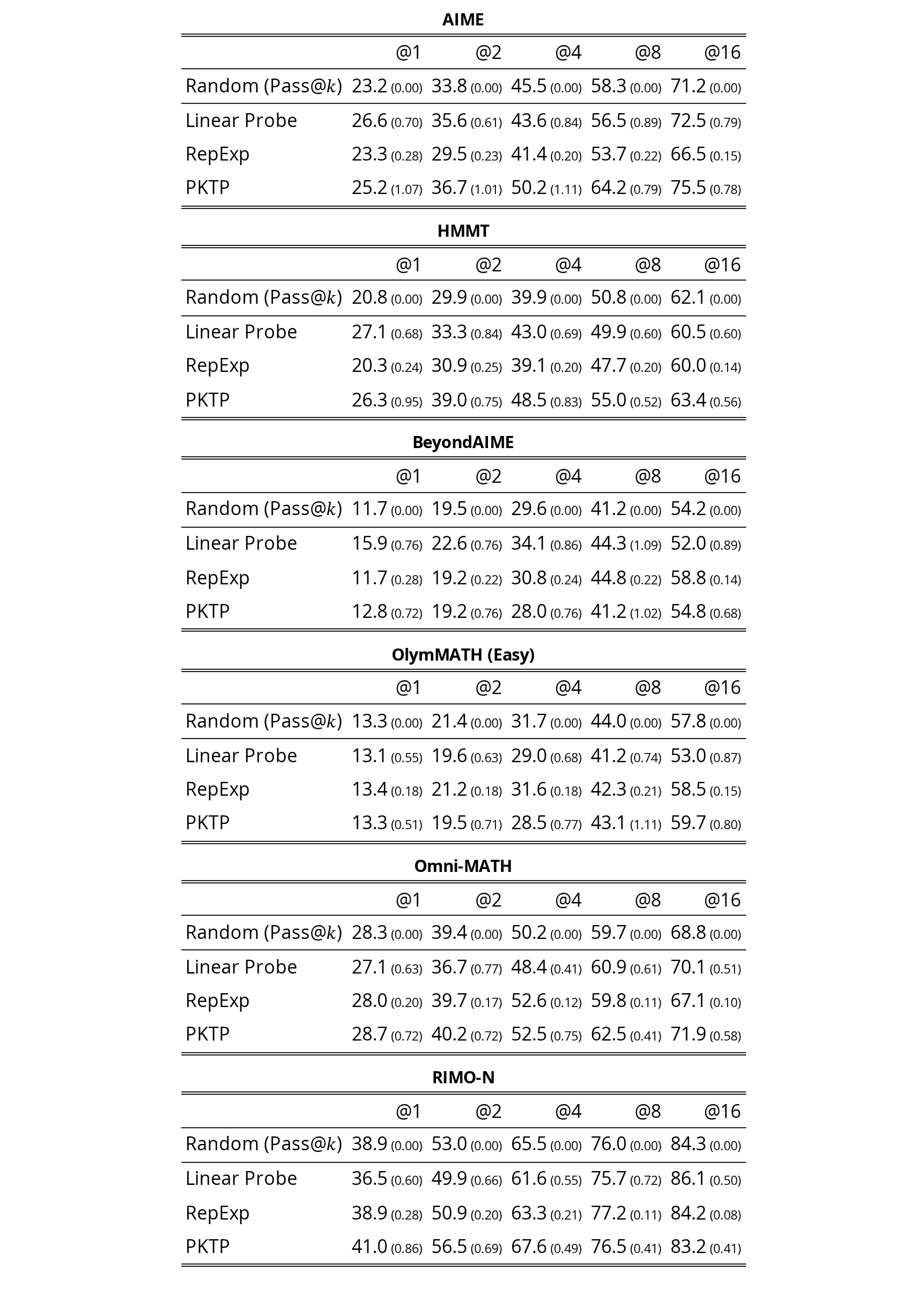
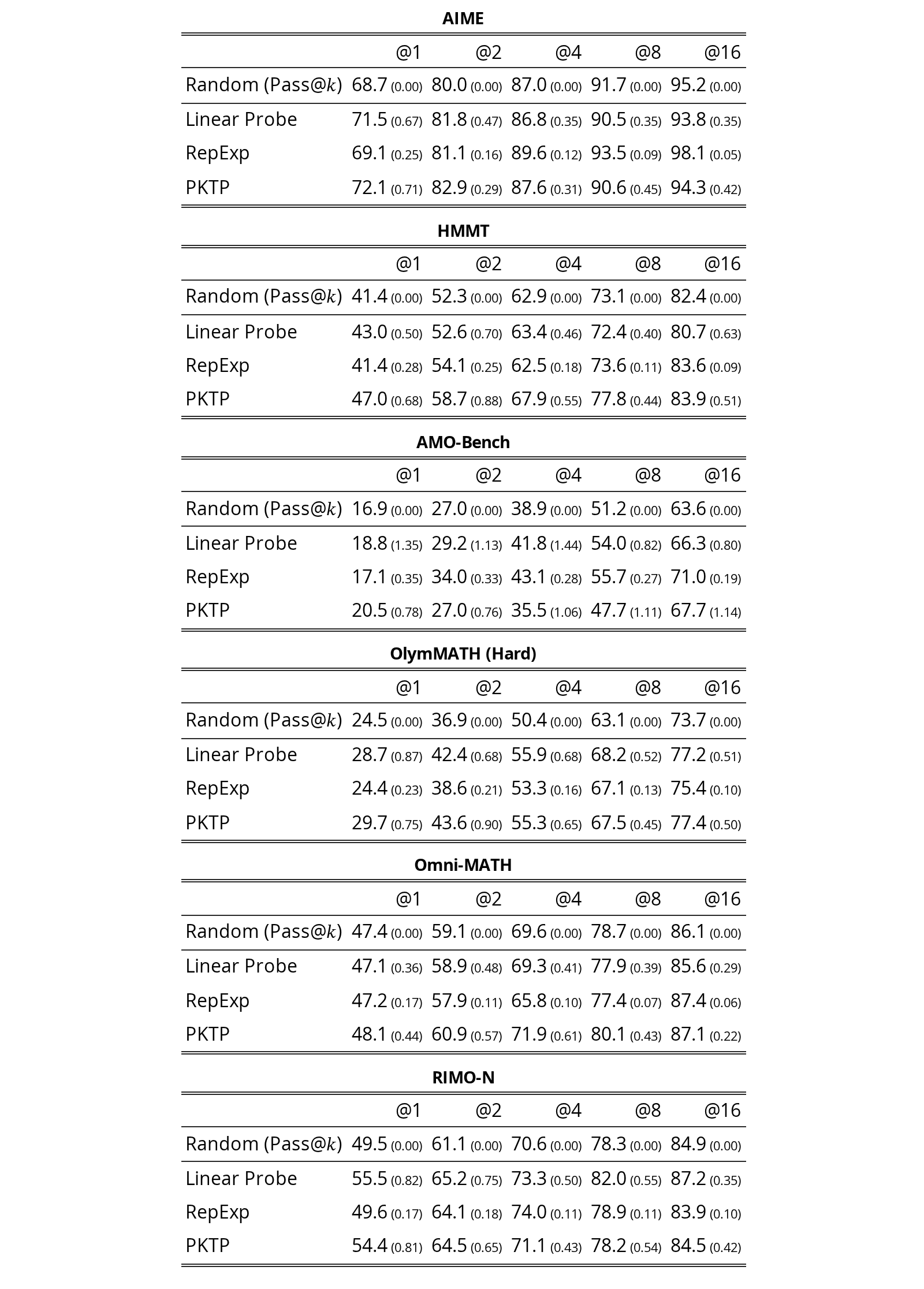
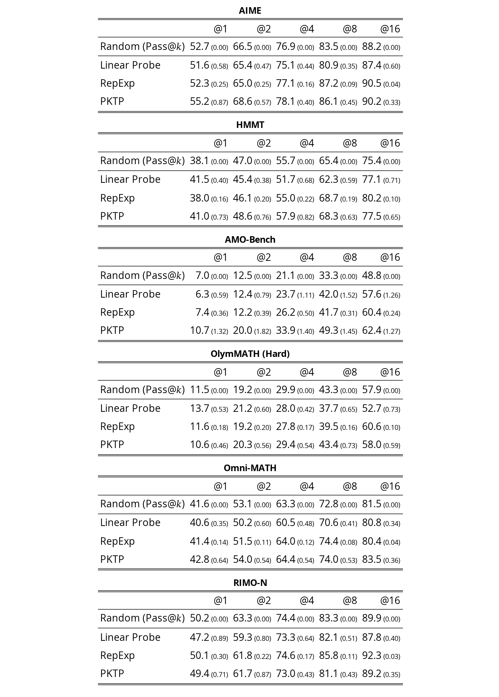
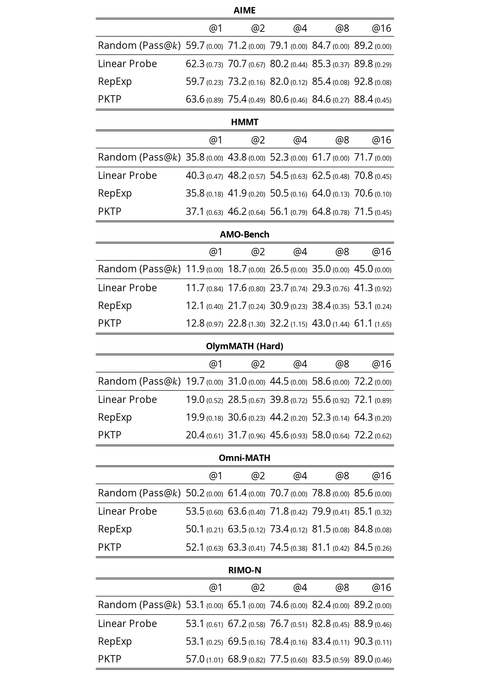
This section reports the numbers behind Fig. 3. Table 1 gives, for every model, the of each pruning policy pooled over all test problems, and Tables 2 to 9 break these results down by benchmark, one table per model. All tables use the setting of Section 4.1, with a pool of rollouts, a cutoff of tokens and eight-fold cross-validation repeated times. Each entry is the average over the repetitions, in percent, and the value in parentheses is its standard error over those repetitions.
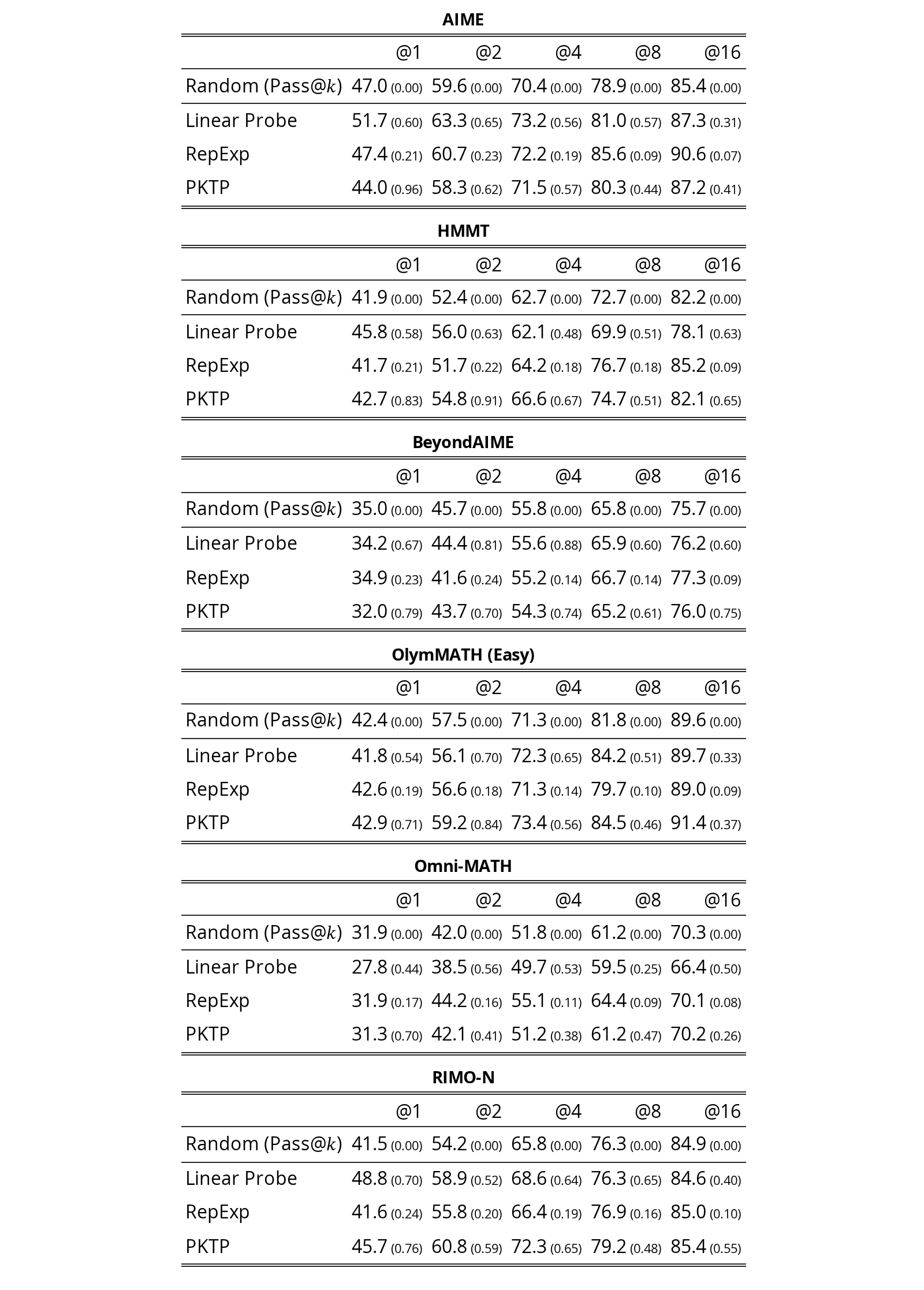
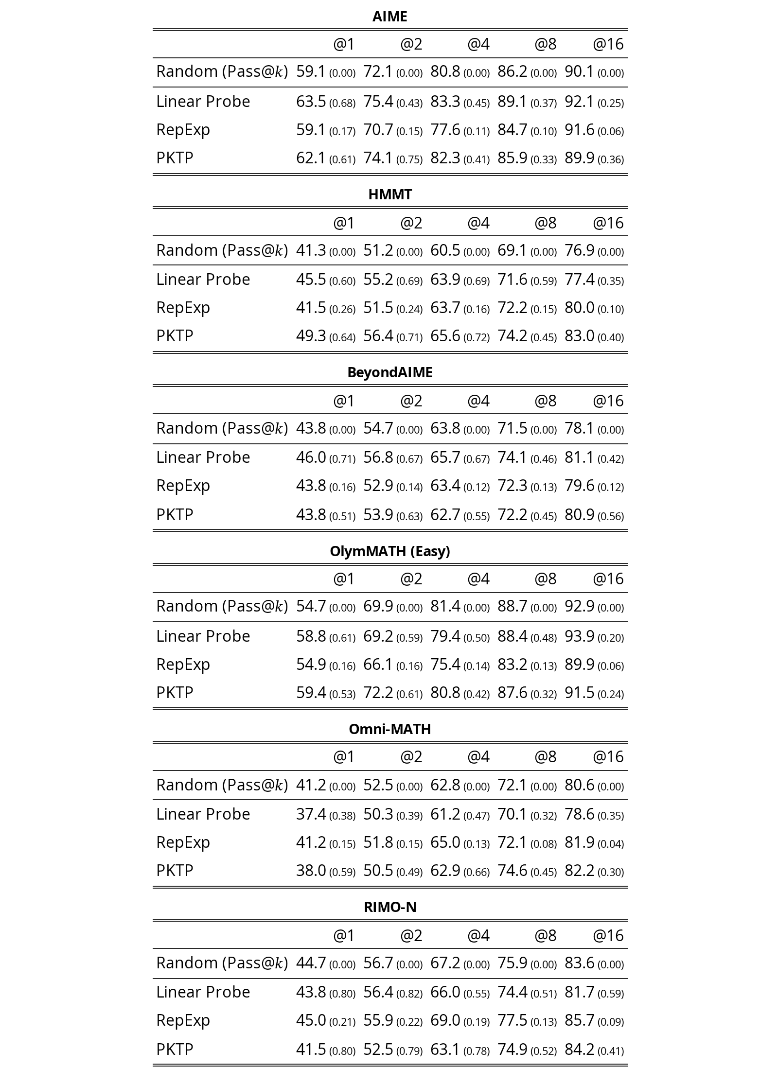
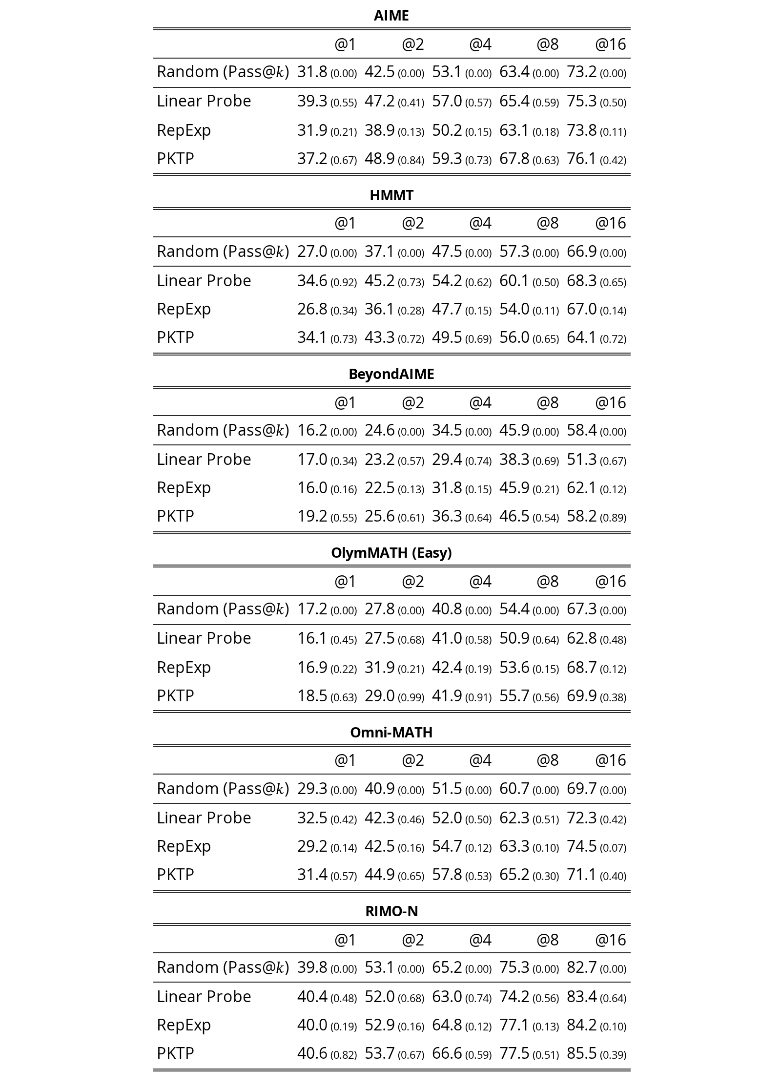
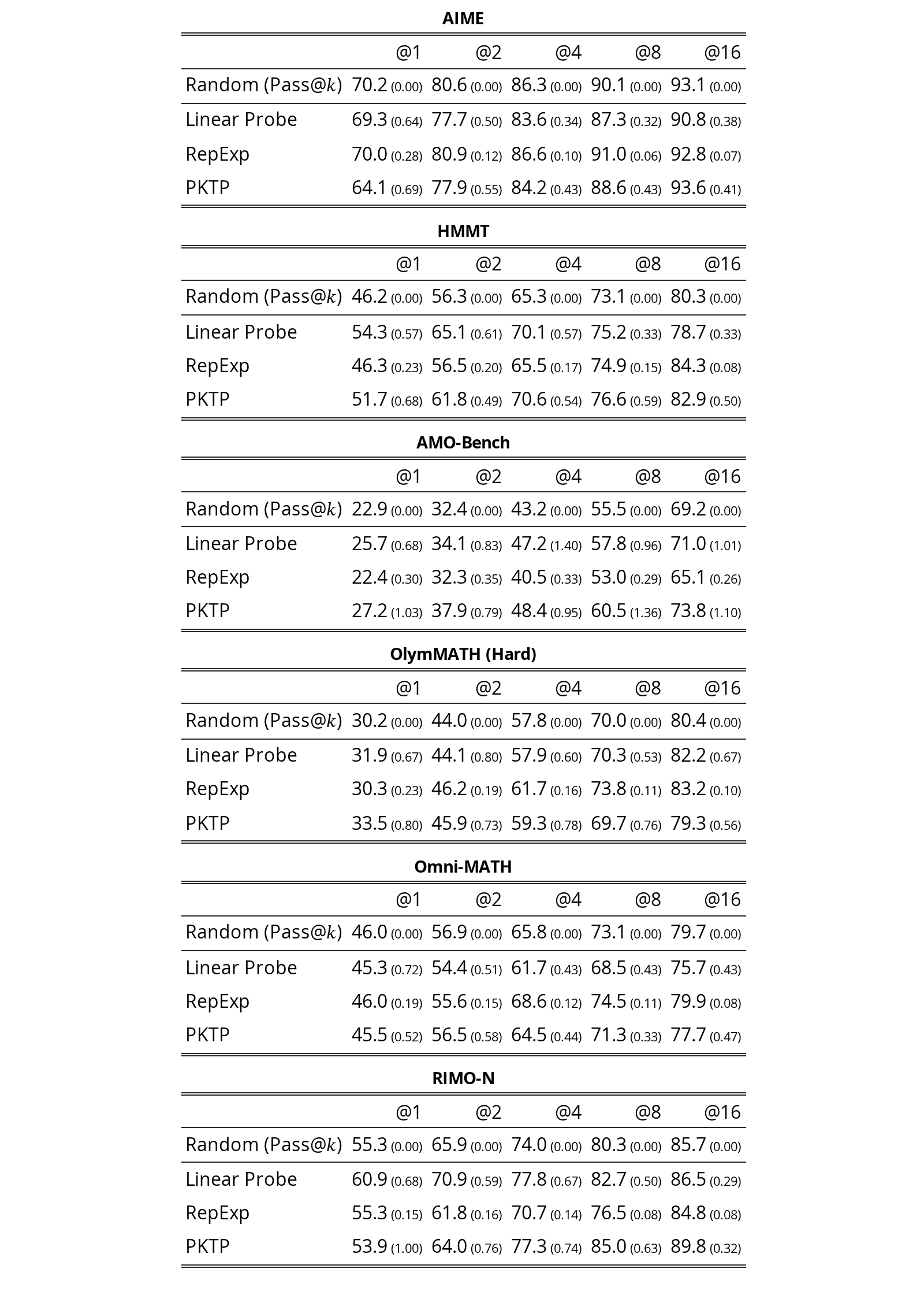
This section repeats Fig. 3 for the other pool sizes, , where the pool of each problem is drawn from its generated rollouts and the cutoff is as in the main setting.
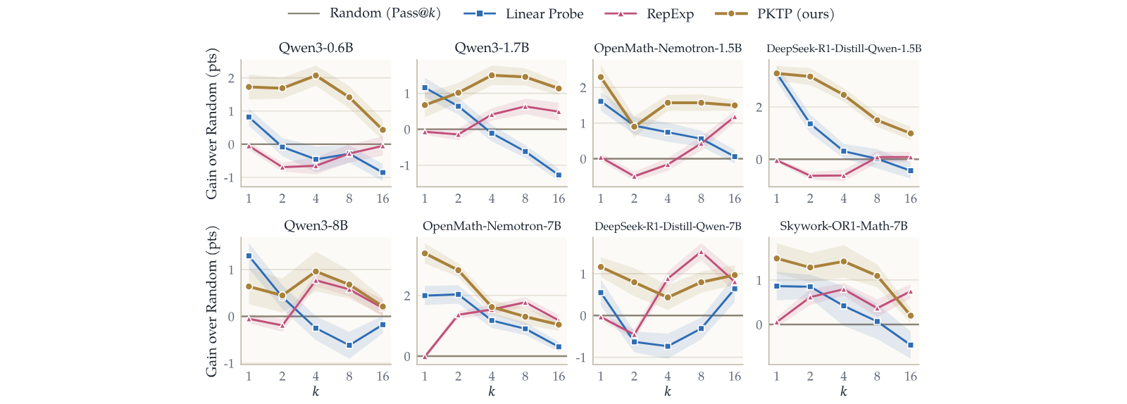
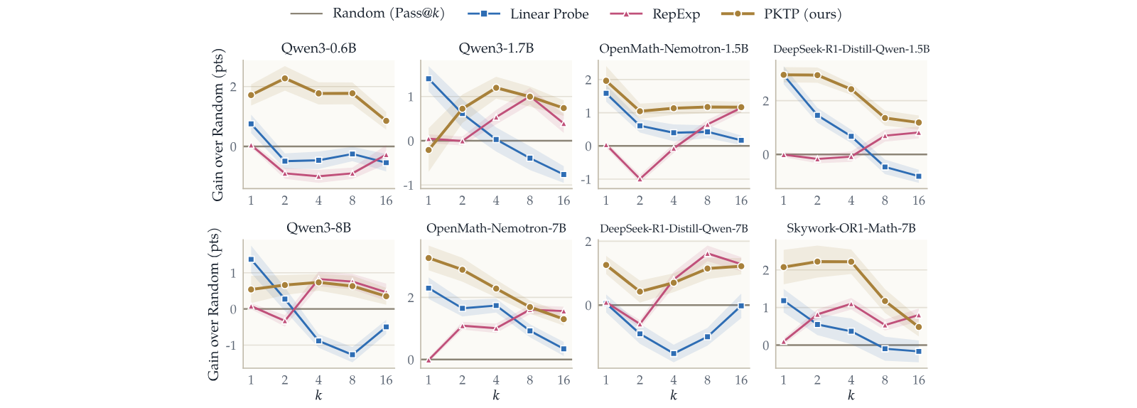
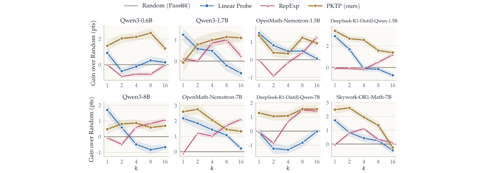
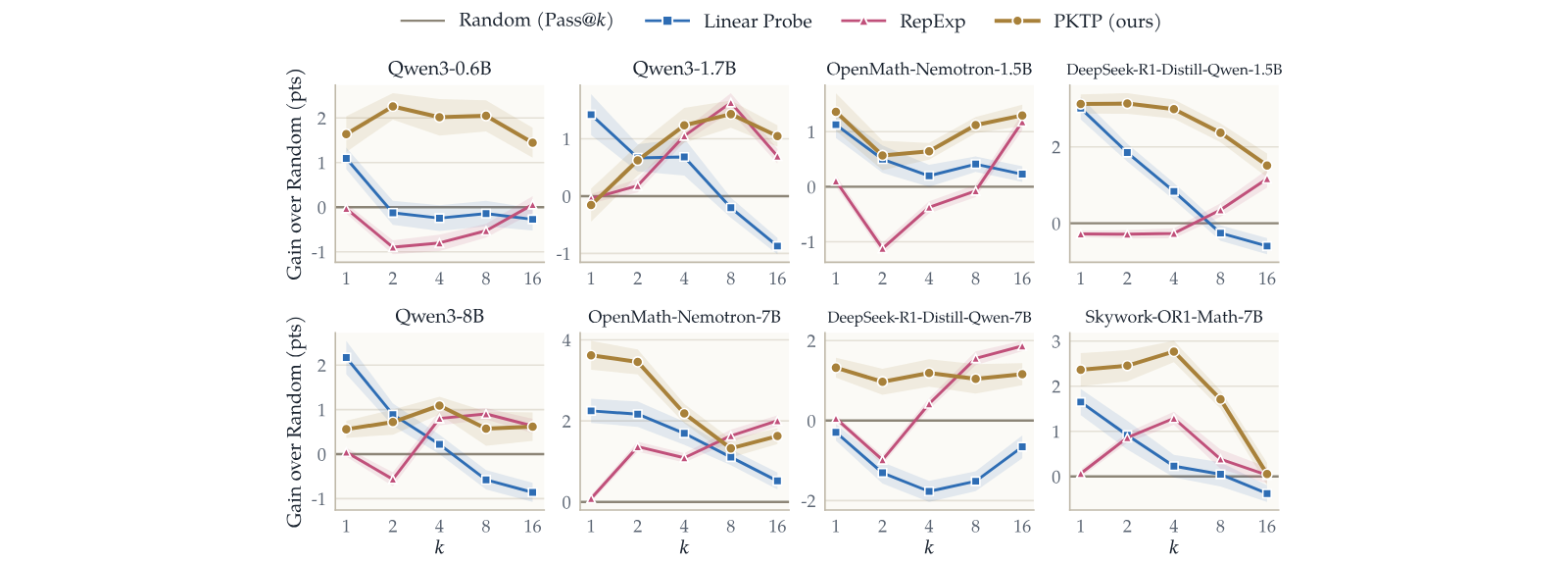
For each rollout, let be the hidden state of the last transformer block of the model at the -th generated token, where is the hidden size of the model, which is for Qwen3-0.6B, for Qwen3-1.7B, for Qwen3-8B, for OpenMath-Nemotron-1.5B and DeepSeek-R1-Distill-Qwen-1.5B, and for OpenMath-Nemotron-7B, DeepSeek-R1-Distill-Qwen-7B and Skywork-OR1-Math-7B. The EMA follows with , and is the normalized value of after the first generated tokens, or after all of them for a rollout that ends before the cutoff.
Test-time scaling generates many rollouts per problem and aggregates them [44, 3, 35, 48], and a growing line of work saves compute by stopping unpromising rollouts early. One family uses the model’s own confidence, such as token-level confidence or its self-estimate of success, to decide which rollouts to continue [30, 13]. Another scores partial rollouts with a reward model [36] or with a probe on the hidden states [54, 1, 25]. Yang et al. 51 concurrently use such a probe for a beam search over partial rollouts, pruning weak rollouts and branching new rollouts from the best prefixes. All of these score each rollout on its own and keep the highest-scoring ones, which is the pure exploitation extreme of Section 2. At the other extreme, RepExp [39] selects rollouts whose representations are least explained by those already chosen, without using their quality. PKTP sits between the two, since it models how the outcomes of the rollouts depend on each other and chooses the set with the highest predicted .
Pass@ is a standard evaluation metric for reasoning and code generation, and several works optimize it during training. Walder and Karkhanis 41 derive low-variance policy-gradient estimators for , Chen et al. 8 use as the reward to balance exploration and exploitation, and Chow et al. 10 fine-tune a model for best-of- inference. Chen et al. 7 reward a group of responses for both quality and diversity, measuring diversity by the determinant of their similarity matrix. These are post-training methods, while PKTP leaves the model unchanged and optimizes at inference time by choosing which partial rollouts to continue. Concurrently, Wu et al. 47 also leave the reasoning model unchanged, but use as the reward to train a planner that writes a different outline for each rollout before it is generated. They thus change how the rollouts are sampled, while PKTP takes independently sampled partial rollouts as given and chooses which of them to continue.
The same objective appears in information retrieval as the expected 1-call@, the probability that at least one of the top documents is relevant. Chen and Karger 6 optimize it greedily, and Sanner et al. 34 show that greedy optimization under a latent subtopic model of relevance leads to diverse rankings, in the same way that our latent factor leads to diverse kept sets. In Bayesian optimization, the batch probability of improvement is the probability that at least one point of a batch improves on the incumbent, and it is monotone and submodular, so it can be maximized greedily [46, 32]. Other methods balance quality and diversity with a hand-set trade-off, such as maximal marginal relevance [5] and determinantal point processes [22]. In contrast to these works, PKTP applies to partial reasoning rollouts, learns the joint distribution of their outcomes from their representations, and optimizes a closed-form surrogate that keeps the submodularity of the exact objective.