Inverse Modeling for Laser Pulse Shape Design in Inertial Confinement Fusion
arXiv:2610.33096v1 · This workspace stays on this version. Check arXiv for newer versions
Some source details need review 5 to check
Original formulas, table values and figures are preserved. Comparison can miss differences; use the original PDF to check details.
Reading view checked: 571 math expressions, 0 rendering failures; 23 of 23 images available.
Compared 292 of 372 source passages against 31 of 35 PDF pages.
- This long paper was only partially compared; the original sources remain available.
HTML S1_p1_1 says “tools such as LILAC [[19](#bib.bib31), [48](#bib.bib32), [11](#bib.bib33), [30](#bib.bib34), [16](#bib.bib35), [17](#bib.bib36)]”; PDF page 1 reads “tools such as LILAC [ 19 , 47 , 11 , 30 , 16 , 17 ]” and visibly shows 47, contradicting HTML. Check PDF page 1
PDF page 2 reads “denoising diffusion models [21, 44],” while HTML block S2_p4_1 reads “denoising diffusion models [[21](#bib.bib2), [45](#bib.bib3)].” Check PDF page 2
HTML block S3_SS1_SSS1_p1_1 has “physics applications [[34](#bib.bib37), [51](#bib.bib38), [39](#bib.bib39), [43](#bib.bib1)]”; original PDF page 3 reads “physics applications [34, 50, 38, 42]”, visibly contradicting the HTML. Check PDF page 3
HTML A1_p2_1 quotes “AR models [[22](#bib.bib29), [49](#bib.bib30)]”; original PDF page 15 visibly reads “AR models [22, 48]”. The PDF contradicts the HTML citation. Check PDF page 15
23 of 23 figure, table and graphic images captured. Open original PDF
Abstract
The achievement of practical fusion energy remains one of the most pressing unsolved scientific challenges, with immense implications for carbon-free power. A critical factor in the success of Inertial Confinement Fusion (ICF) is the design of a Laser Pulse Shape (LP) that can optimally drive implosions under stringent physical constraints. Traditional LP design relies on computationally expensive simulations and manual iterative refinement. We introduce the ICF Laser Pulse Shape Design System (LPDS), a generative inverse modeling framework that maps desired outcomes and target pellet configurations directly to optimized LPs. Crucially, we design a multi-objective loss function to ensure the generated LPs satisfy fundamental physical constraints and experimental requirements. Furthermore, we present constraint-conditioning, inpainting, and gradient-based LP editing mechanisms for fine-grained control over specific pulse characteristics during generation. Moreover, we study the transfer of our framework to a limited set of real experimental shots. Our method establishes a data-driven inverse design framework for LP design in ICF, contributing to the advancement of practical and sustainable fusion energy.
Inertial Confinement Fusion (ICF) is a promising route toward fusion energy, but it requires precise design of the Laser Pulse Shape (LP), the temporal profile of laser energy that controls target compression. Crafting effective LPs is particularly challenging because implosion performance depends nonlinearly on small changes in pulse timing, amplitude, and target configuration. In the direct-drive setting studied here, LP design relies on repeated radiation-hydrodynamic simulation sweeps and expert iteration with tools such as LILAC [19, 48, 11, 30, 16, 17]. This forward-design process is computationally expensive and limits rapid exploration of promising designs, creating a need for inverse models that map desired outcomes to candidate LPs. In this work, we introduce the Laser Pulse Shape Design System (LPDS), a machine learning-based inverse-modeling framework to address this challenge. LPDS enables scalable, data-driven LP design aligned with target implosion objectives and experimental constraints. The main contributions of our work are:
- •
We propose a unified inverse design framework that jointly integrates closed-loop physics optimization, adaptive constraint reconfiguration, and multi-solution design for ICF.
- •
We propose a constraint-adaptive conditioning mechanism for LP design, enabling rapid reconfiguration to new design constraints without retraining the full generative model.
- •
We formulate a unified multi-objective training scheme combining reconstruction, physics consistency, and energy conservation, allowing controllable trade-offs between diversity and physical fidelity.
- •
We demonstrate generative inverse modeling for LP design in ICF using large-scale simulation data, true LILAC-simulator validation for the best-performing models, and a limited experimental transfer study on 300 experimental shots.
ICF achieves nuclear fusion by using high-energy lasers to compress and heat fuel pellets (typically deuterium-tritium) to extreme temperatures and pressures [6]. Achieving ignition requires precise, symmetric implosion controlled by the LP, the temporal profile governing compression over 3 nanoseconds.
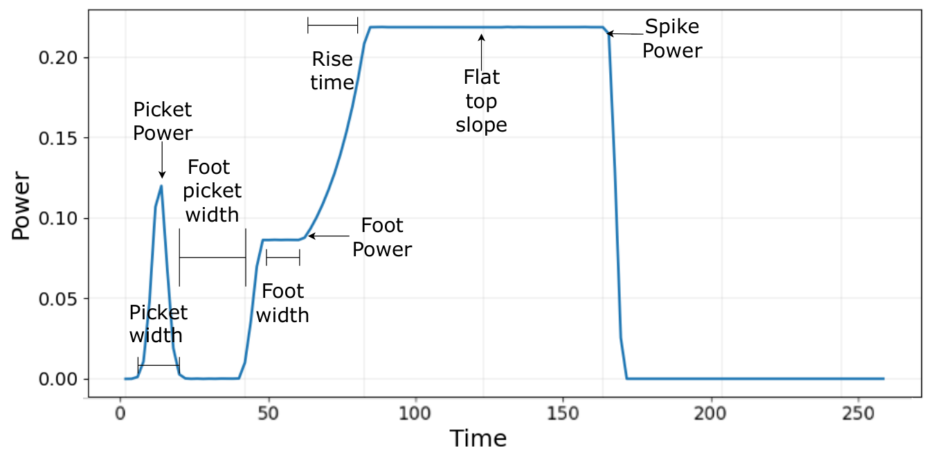
The LP is carefully structured with distinct phases: a low-intensity foot launches timed shocks, a rising ramp controls pressure buildup, a high-intensity main pulse drives rapid implosion, and an optional tail sustains pressure (Figure 4). This multi-phase structure ensures symmetric compression and optimal fusion conditions.
Given the high cost of experiments and limited access to ICF facilities, researchers rely on physics-based simulations to evaluate LP designs. LILAC is a prominent one-dimensional Lagrangian hydrodynamics code for ICF [19, 48, 11, 30, 16, 17] that maps LPs and target parameters to implosion outcomes such as energy yield, velocity, and areal density. This controlled environment enables systematic exploration of how variations in the LP influence fusion performance for a given target.
LPDS builds on two families of generative models: denoising diffusion models [21, 45], and autoregressive sequence models [22, 49]. Their formal definitions are provided in Appendix A. The iterative denoising process of diffusion models provides a natural mechanism for controlling multi-scale pulse features, while autoregressive models capture the sequential temporal structure of the LP.
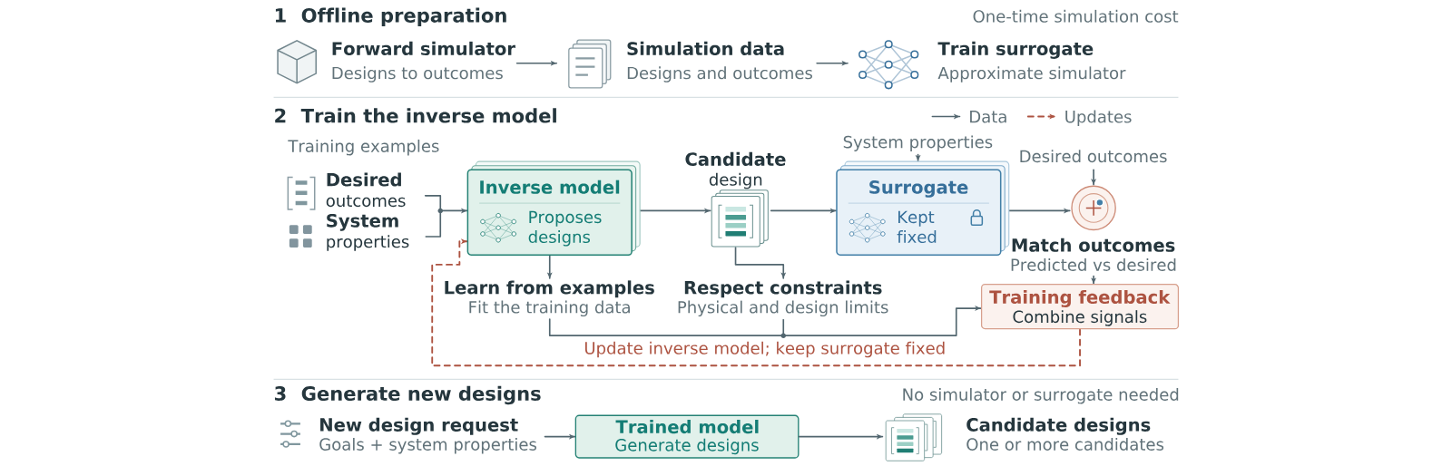
We present LPDS, an inverse-modeling framework for generating LPs in ICF. LPDS takes desired implosion outcomes and target pellet parameters as input and generates LPs that satisfy the specified fusion objectives. Figure 1 summarizes the workflow: offline simulation and surrogate training (1), physics-guided inverse-model training (2), and direct design generation (3). In our ICF application, designs are laser pulses, system properties are pellet parameters, and outcomes are implosion metrics. The following subsections describe each component of LPDS in detail.
Let denote the vector of implosion outcomes produced by the LILAC ICF simulator for a given LP () and target pellet parameters (). These outcomes include quantities such as energy yield, areal density, burn width, and ion temperature. The pellet parameters are defined by attributes such as outer radius, ice thickness, ablator thickness, and ice-tritium fraction.
To construct an inverse design model, we first generate a dataset of 1 million examples via systematic simulation sweeps, capturing the relationship between pulse shapes, target parameters, and resulting implosion outcomes. The LP is represented as a real-valued sequence of length 256. and are real-valued vectors of size 5 and 12, respectively. The underlying simulation inputs live in a 20-dimensional design space that combines target specifications with an internal parameterization of the pulse shape; to sample high-value regions of this space efficiently, we combine random physically valid draws with perturbations of known high-performing implosions.
Our goal is to learn a data-driven inverse model conditioned on desired implosion outcomes and pellet parameters . For stochastic generators, this corresponds to learning a conditional distribution from which candidate LPs can be sampled; for deterministic predictors, it corresponds to learning a point estimate . In the terminology of simulation-based inference, the stochastic variants are amortized neural posterior estimators [9]: because LILAC is too expensive to query during training or inference, LPDS learns the posterior from a fixed set of simulations and is then applied to new targets without further simulator calls. For simplicity, we denote a generated candidate pulse by:
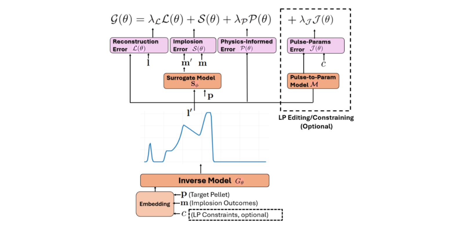
Conditioning parameters and are linearly embedded before entering ; Appendix Figure 3 shows the ICF-specific architecture and optional pulse-shape constraints.
This inverse design problem has multiple plausible solutions, since multiple pulse shapes can lead to similar outcomes. To address this, we consider two modeling approaches:
- •
Generative (Stochastic): Diffusion and autoregressive generative models are trained to sample from a distribution of valid LPs, thereby providing diversity and robustness.
- •
Predictive (Deterministic): We also train predictive autoregressive models to predict a single high-fidelity LP.
Diffusion models iteratively denoise a latent representation to sample from a learned distribution. This property has made them increasingly attractive for physics applications [34, 51, 39, 43].
We condition on both the desired implosion outcomes and the target parameters . During the forward diffusion process, noise is gradually added to the original LP over timesteps, resulting in a noisy latent variable . The inverse model learns a conditional noise prediction network that estimates the noise added during a forward process, conditioned on the noisy LP , the timestep , the target implosion outcomes , and the target parameters . The training objective of the network is:
During the generation phase, we start from a random noise vector and iteratively denoise it using the conditional noise prediction network via the DDIM [45] update rule:
where is estimated via:
With this diffusion-based formulation, LPDS generates diverse LPs that remain consistent with target constraints, enabling systematic exploration of physically meaningful designs.
Alternatively, LP design can be formulated autoregressively, with the pulse vector generated sequentially. At each timestep , the model predicts conditioned on the target parameters , the desired implosion outcomes , and the previously generated pulse values . This formulation allows the model to capture the temporal dependencies inherent in the pulse sequence. At the first timestep, when no previous values are available, the model conditions on an initialization vector obtained by projecting the target parameters and desired outcomes into a shared embedding space. This embedding serves as the initial conditioning input for the autoregressive model.
We explore two paradigms for the autoregressive models: predictive and generative. The predictive models reconstruct the ground-truth LP with high fidelity, whereas the generative models trade off reconstruction fidelity against the ability to provide diverse LP candidates. The training objective for the predictive autoregressive models is the mean squared error between the predicted and true pulse values across all time steps:
where denotes the model’s prediction for timestep given the prior pulse values and conditioning inputs.
At each time step, the generative models output a probability distribution over the LP value at time denoted by . The training objective for the generative autoregressive models is to minimize the negative log-likelihood of the true pulse under the predicted distribution :
We explore three modeling choices for . The simplest models it as a Gaussian distribution, in which predicts the mean and variance. To provide greater expressiveness, we also model as a weighted mixture of Gaussians, where the model predicts -dimensional vectors for the means, variances, and mixing weights. Finally, we consider a discrete approach in which the pulse is quantized into 128 values and is modeled as a categorical distribution trained with a cross-entropy loss.
While the reconstruction objective enables LP reproduction, our broader goal is scientific exploration through plausible, diverse LP generation consistent with implosion outcomes. This provides a wider array of selectable, high-performing candidates and facilitates scientific discovery by potentially identifying novel LP configurations. To achieve this, we integrate a differentiable physics surrogate directly into the generative training loop.
From an optimization perspective, this process can be viewed as a bilevel problem in which a generative model proposes candidate designs while a physics model evaluates their feasibility and performance. LPDS approximates this process by optimizing the inverse model end to end through a frozen differentiable surrogate, directly aligning the generative distribution with the physically valid solution manifold. By incorporating differentiable physics surrogates into the training loop, the model does not merely condition on observed data but actively optimizes generated designs toward target physical outcomes.
For this purpose, we train a surrogate model to approximate the LILAC simulator. This model learns the mapping from an LP and target parameters to the corresponding implosion outcomes . This can be represented as , where represents the learnable parameters of the surrogate model. The surrogate is trained on the simulation dataset by minimizing the prediction error:
After training, is kept frozen and is used during training of the inverse model to evaluate the physical fidelity of generated LPs. Given a generated pulse , the surrogate model predicts the corresponding outcomes , which are then compared to the target outcomes . Our new objective can be defined as:
Here, and control the trade-off between faithfully reconstructing the original LP and generating physically consistent alternatives. Properly tuning these weights allows the model to generalize beyond pure reconstruction, producing diverse yet plausible LPs tailored to the specified design goals. In practice, we first train only on the reconstruction loss since at the beginning of training can produce LPs that are incoherent and out-of-distribution for .
For our diffusion model, this loss formulation appears to require knowledge of the clean LP at each reverse step. However, DDIM’s non-Markovian formulation allows us to estimate at any intermediate timestep using Equation 5.
While our goal is to generate a diverse set of LPs for a given target configuration, the practical utility of these designs depends critically on their adherence to the fundamental physics of ICF and their feasibility under real-world experimental constraints. One essential constraint is energy conservation. Specifically, generated LPs should not exceed the total energy budget of corresponding reference pulses. For any , we impose the following constraint on a generated LP :
where is the total pulse duration. To enforce this, we introduce a physics-based penalty term:
This term penalizes excess energy, encouraging designs within experimental and physical limits. Incorporating this constraint into our overall loss function, we define the complete training objective as:
where , , and are hyperparameters that control the relative importance of each loss term in the overall objective (Ablation of in Appendix Section E.1). This joint objective enables the generation of LPs that are diverse, outcome-consistent, physically plausible, and experimentally viable.
We compare LPDS variants across deterministic models (an autoregressive Transformer [49], , and an LSTM [22], ) and generative models (a diffusion model, , and three autoregressive LSTM variants with Gaussian, Mixture-of-Gaussians, and categorical output distributions). A comparison against seven off-the-shelf conditional generators and inverse-problem methods is reported in Appendix D, and generalization to unseen pellet configurations is evaluated in Appendix E.3.
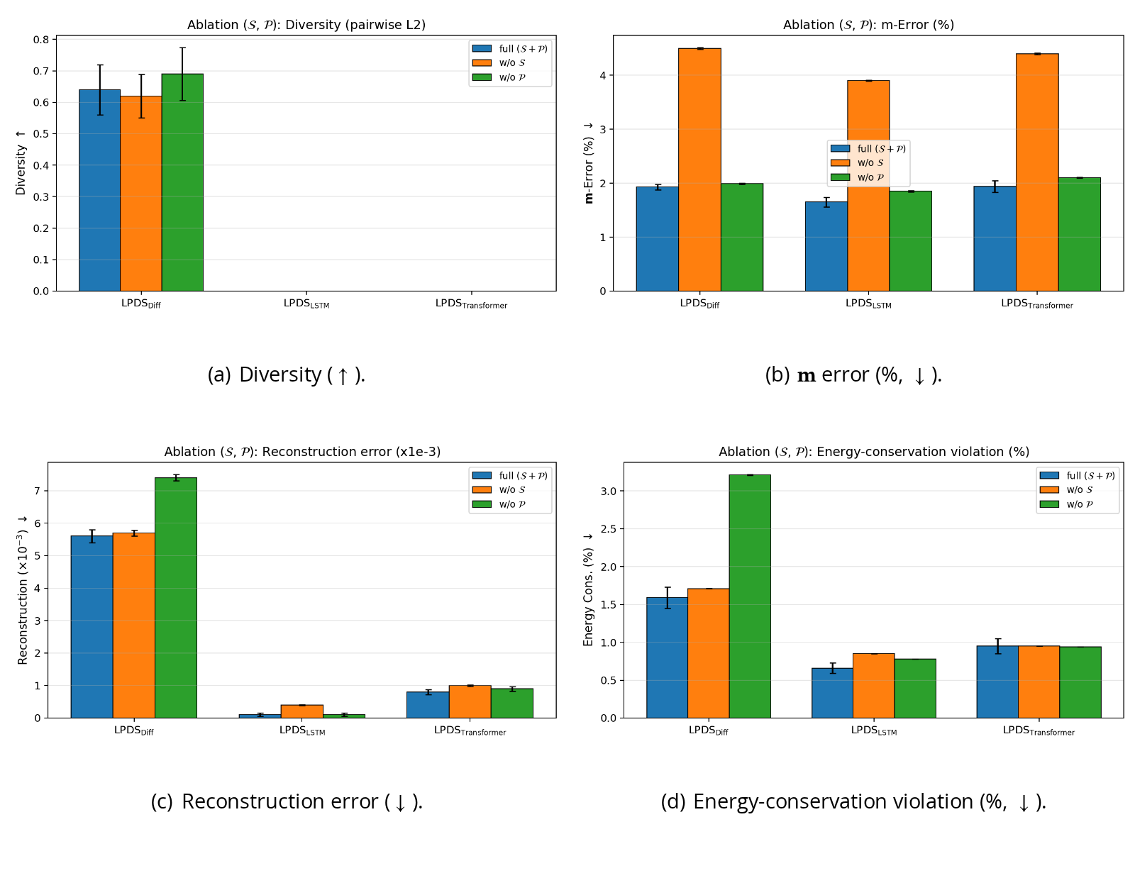
We also perform an ablation study to assess the impact of our proposed objectives by evaluating versions of the model without the surrogate loss () and without the physics-informed loss ().
We report four key metrics: implosion-outcome error in , reconstruction error, generation diversity, and energy-conservation violation. All models were evaluated over full training runs and random seeds (50 runs per model) on a test set , where .
The implosion-outcome error in is computed via the surrogate loss (Equation 10) and reported as mean absolute percentage error (MAPE). Reconstruction error is computed as . Energy-conservation violation is reported as the mean positive excess-energy percentage, , so lower values indicate fewer budget violations. Diversity is measured by average pairwise distance across generated samples: . The estimated upper bound for diversity is , obtained when comparing randomly selected LPs from .
We also evaluate the implosion-outcome error on the true LILAC simulator, rather than relying only on the surrogate, and report this quantity as the LILAC error. Because simulator access is limited, this validation is performed for the two best-performing models ( and ). The LILAC error therefore serves as the primary simulator-grounded validation of LPDS and should not be conflated with surrogate-based screening.
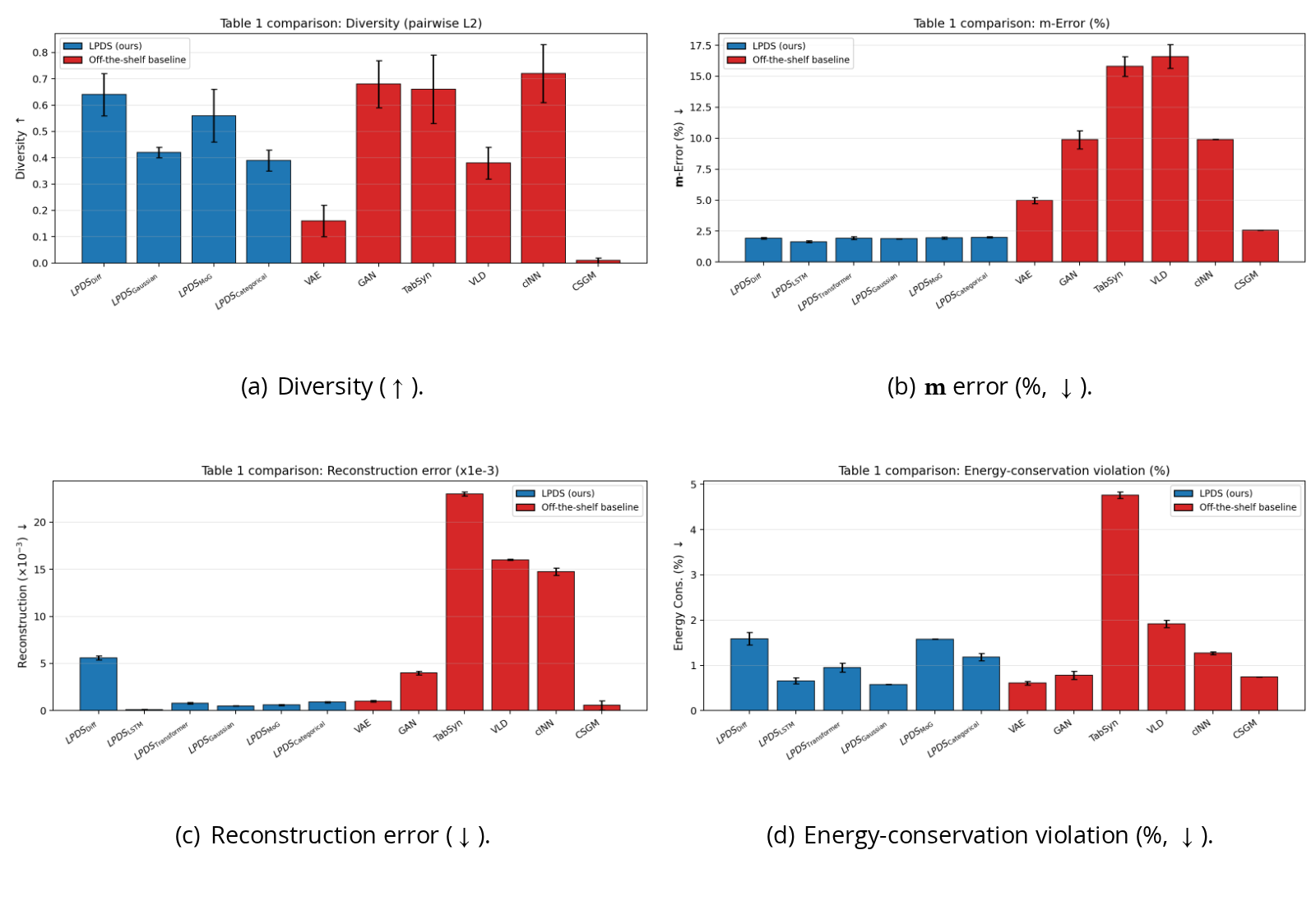
Table 1 summarizes the main results. The ablation studies confirm the critical roles of and . Among LPDS variants, achieves the highest reconstruction fidelity but yields zero diversity. The generative variants ( and ) maintain low implosion-outcome error while producing varied, high-quality pulses (Figure 2a), with providing the greatest diversity while preserving low error. This precision–diversity trade-off enables scientists to select predictive models for exact replication or generative models for constraint-driven exploration; example generations are shown in Appendix Figures 9(b)–11(b). The two best variants ( and ) both achieve less than error on the true LILAC simulator, confirming that surrogate-based gains transfer to the simulator. Per-metric bar plots of these results are provided in Appendix D (Figures 5 and 6).
| LPDS variant | Diversity | Error | Reconstruction | Energy Cons. | LILAC Error |
|---|---|---|---|---|---|
| (%) | () | (%) | (%) | ||
| Diff | |||||
| LSTM | – | ||||
| Transformer | – | – | |||
| LSTM | – | ||||
| LSTM | – | ||||
| LSTM | – | ||||
| Diff w/o | – | ||||
| LSTM w/o | – | – | |||
| Transformer w/o | – | – | |||
| Diff w/o | – | ||||
| LSTM w/o | – | – | |||
| Transformer w/o | – | – |
View original table
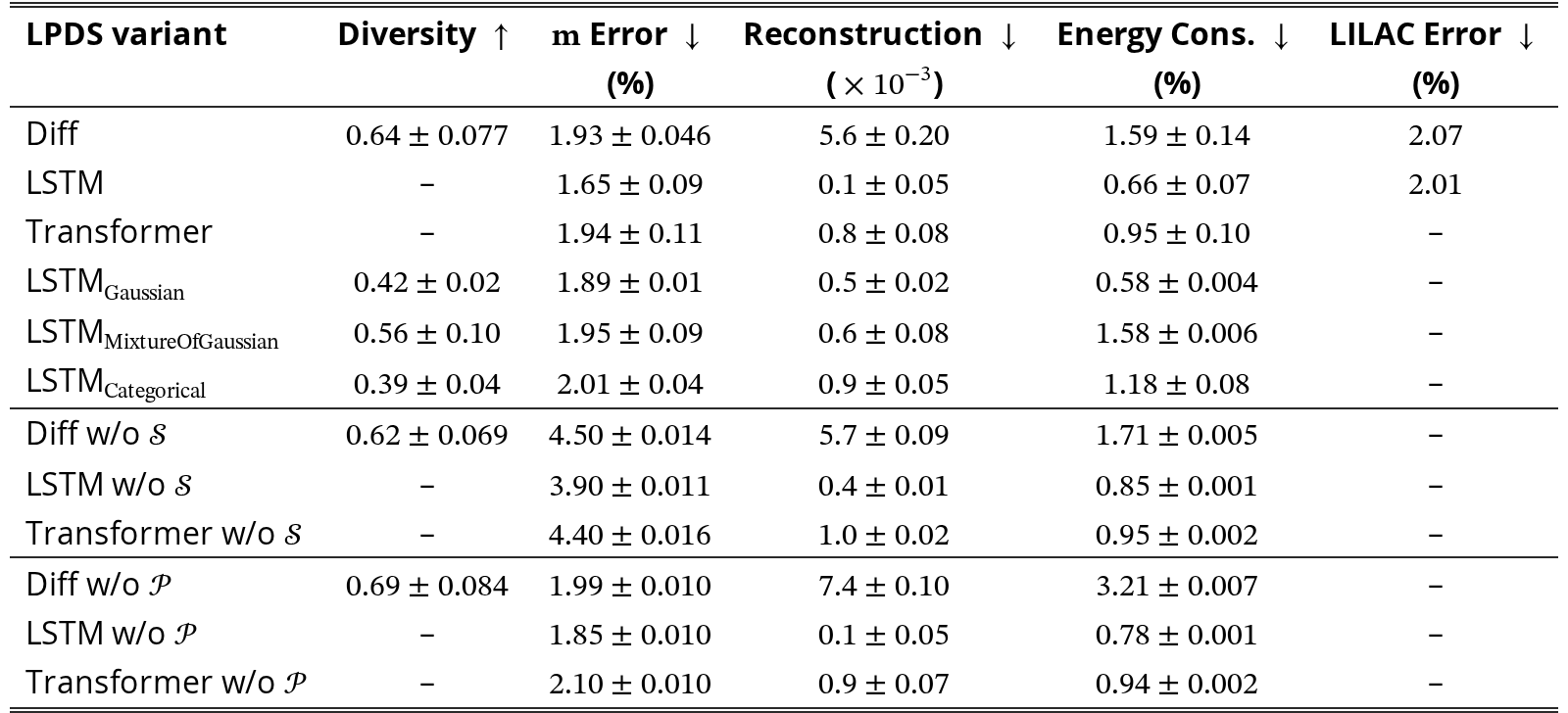
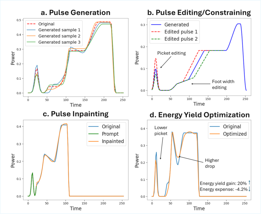
Figure 2 illustrates the generation, editing, inpainting, and optimization capabilities supported by LPDS.
In many ICF design scenarios, scientists require control over specific regions or attributes of the LP. We use a mapping function , implemented as an LSTM trained on the same dataset (details in Appendix B.2), to project an LP onto parameters . Each corresponds to a physically interpretable property of the LP (Figure 4). When constructing new designs, scientists may fix one or two of these values while allowing the remaining parameters, and thus the overall pulse shape, to vary.
However, our current inverse model lacks a mechanism to enforce such partial constraints during inference. A straightforward solution would be to take the constraint parameter as an additional input during training, producing an LP conditioned on the desired implosion outcomes , target parameters , and the specified constraint as . A constraining loss can then be introduced to enforce consistency between the specified constraint values and their corresponding values in the generated LP:
where . The constrained objective can be defined as:
The above approach enables to satisfy the specified constraints. However, exhaustively training separate diffusion models for all combinations of one or two parameters in is computationally infeasible due to combinatorial complexity.
To address this challenge, we propose a rapid adaptation strategy [5, 37, 14, 23]. Rather than retraining from scratch, we adapt a pre-trained model with a small number of gradient updates to satisfy a new constraint .
Our adaptation approach employs an embedding network that encodes constraint parameters to condition LP generation. This results in a conditioned noise model: . To simplify conditioning, we enforce equal embedding dimensionality for and , enabling their combination into a single conditioning variable . This allows us to condition the model as , requiring no architectural changes to the original model. During adaptation, only the parameters of are fine-tuned, according to Equation 14, while the remaining weights are frozen.
Conceptually, the proposed adaptation mechanism can be interpreted as learning a low-dimensional constraint embedding that shifts the generative distribution toward constraint-satisfying submanifolds. Rather than retraining the full generative model for each new constraint configuration, LPDS performs lightweight updates that reconfigure the generative process while preserving the learned global structure of the design space.
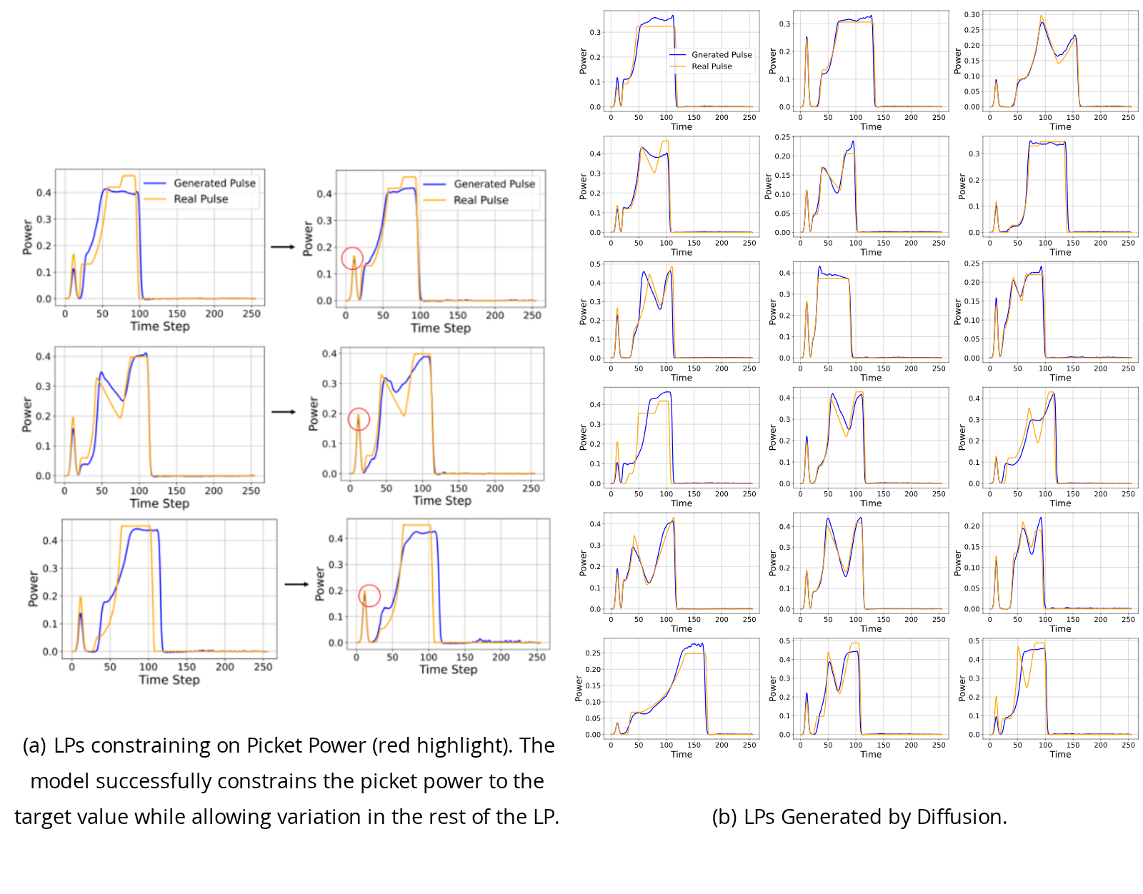
Examples of this adaptation technique for picket power are shown in Figure 9(a) (Appendix). For a given constraint , the model is fine-tuned once and can then generate an arbitrary number of pulses for different specifications of and .
Alternatively, the LP can be adapted after generation using a model-agnostic technique without additional fine-tuning. To honor constraints in while maintaining desired implosion outcomes, a loss combining the pulse constraining loss (Equation 13) and the LILAC surrogate loss (Equation 10) is formulated. Since both losses are differentiable w.r.t. the pulse (now referred to as and ), we can perform gradient descent with respect to the following loss and update the pulse :
where is the learning rate. One drawback of this technique is that gradient descent can push the LP into undesirable regions, such as negative values or peaks that violate the maximum power. In practice, we mitigate these issues by clipping the pulse. In addition, gradient-based adaptation must be performed separately for each constrained LP, whereas our diffusion-based adaptation produces a fine-tuned model that can be reused indefinitely.
We evaluate the ability of LPDS to rapidly adapt to specific design constraints , using both diffusion-based and gradient-based adaptation strategies. For the diffusion-based approach, the model is fine-tuned for only 10 epochs on a new constraint parameter , requiring minimal computational overhead. In parallel, we apply the gradient-based adaptation to the deterministic model , allowing for direct post-generation refinement.
We focus our evaluation on two physically meaningful parameters: picket power and foot power (see Figure 4). To quantify adaptation accuracy, we compute the mean absolute percentage error (MAPE) between the specified constraint value and the corresponding value extracted from the generated pulse (as defined in Equation 13). The gradient-based approach achieves a MAPE of , while the diffusion-based method yields a MAPE of . Importantly, both adaptation methods preserve LPDS’s performance on the target implosion outcomes (-Error remains unaffected).
These constraint adaptation strategies empower scientists to generate diverse, high-quality pulse shapes that meet desired implosion outcomes and can be interactively tuned to satisfy evolving experimental or engineering constraints.
Inpainting provides control directly in LP space: users specify a prefix or fixed regions rather than parameters in . Autoregressive models complete the pulse from a supplied prefix, while diffusion conditions denoising on specified segments. In our evaluation, the autoregressive prompt covers the first 10% of the pulse (the first peak); diffusion receives random observed segments with the remainder masked. Diffusion and LSTM achieve errors of and , respectively, with reconstruction errors of and ( denotes standard deviation over seeds). Appendix Figures 8(a) and 8(b) show example completions.
Beyond reconstructing existing pulse shapes, LPDS can discover novel laser pulse designs that improve implosion performance under strict physical constraints. We formulate pulse optimization as a constrained generative inverse-design problem in which the goal is to generate new pulse shapes that outperform high-quality baseline designs while preserving energy feasibility.
Specifically, given an initial high-performing pulse with system parameters and measured implosion outcomes , we define a target outcome by increasing the energy yield component by 10%:
Using this target, LPDS generates candidate optimized pulses via
The generated pulse must satisfy two constraints: (i) achieving a predicted energy yield at least as high as the target and (ii) maintaining the original total energy budget,
Here, denotes the surrogate model used to estimate implosion performance. Since the generated LP may lie beyond the physically viable distribution, we further impose a frequency-domain similarity constraint to ensure the generated LPs are physically plausible:
where is the discrete Fourier transform, is the number of temporal samples and controls the allowable structural deviation. This constraint ensures that LPDS explores novel yet physically realistic pulse variations within the learned design manifold.
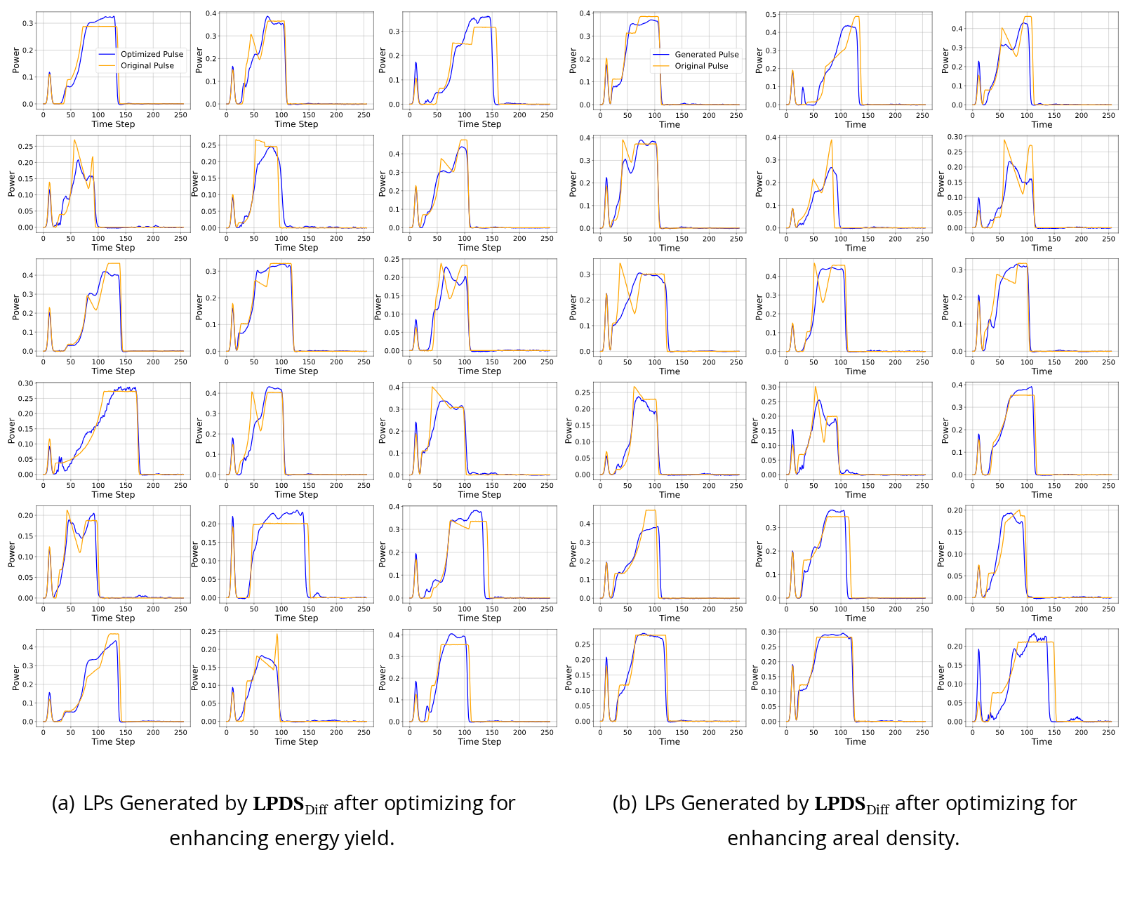
For each initial design, we generate 20 candidate pulses using different random seeds and select the pulse that maximizes predicted energy gain while satisfying all constraints. Crucially, the final optimization results are not reported through the surrogate: the selected optimized pulses are evaluated with the true LILAC hydrodynamic simulator on 60 unique high-performing baseline pulses.
We compare the diffusion-based generator with the autoregressive variant . Under true LILAC validation, the autoregressive model achieves a modest mean energy-yield improvement of 2.79%. In contrast, consistently discovers novel pulse structures that produce a substantially higher mean gain of 17.74% while respecting the original energy budget, and 86% of the optimized pulses exceed the 10% yield-improvement target. A mean gain of corresponds to 1.18 neutron yield, obtained on top of baseline pulses that are already high-performing. These results demonstrate that LPDS can effectively explore the constrained design space and uncover superior pulse configurations beyond the baseline designs.
Real-world ICF data are scarce because experiments are expensive and limited in number. To assess transferability beyond simulation, we conduct a limited transfer study on historical experimental data; this is a retrospective evaluation rather than a prospective facility experiment. We fine-tune LPDS on 300 experimental laser pulses, comprising the complete set recorded to date, using a 70%–30% train–test split. Despite the limited sample size, measurement noise, and domain shift, the surrogate achieves 8% test prediction error. On the experimental test set, LPDS achieves:
- •
an implosion-outcome error of ,
- •
a reconstruction error of , and
- •
an energy conservation error of .
These results are broadly consistent with simulation performance, particularly in reconstruction quality and physical plausibility. The higher -Error is expected given experimental noise and surrogate limitations in this regime. Overall, LPDS shows encouraging transfer from simulation to experiment with minimal fine-tuning; prospective validation on new facility shots remains future work.
ML-based inverse modeling spans diffusion models [10, 8, 25, 46], autoregressive sequence models [12, 36, 52], GANs and VAEs [42, 3, 28, 35], and other paradigms [50, 26, 1]. In the physical sciences, inverse methods have been applied to thermodynamics [24], materials discovery [47, 18], geophysics [40], and high-energy/plasma physics [43, 13, 31, 38]. However, these methods are typically domain-specific and focus on reconstructive inverse problems under fixed forward operators, producing single or narrowly distributed solutions. Simulation-based inference [9] provides a general framework for amortized posterior estimation with expensive simulators, but neural posterior estimators are typically applied to low-dimensional parameter vectors and do not natively address three requirements of LP design: a 256-dimensional structured output, hard physical constraints that must hold for every sample, and interactive control through inpainting and editing. Flow matching [33] is a further generative family that could in principle be combined with the surrogate coupling, energy penalty, and inpainting used in LPDS; we leave its evaluation to future work.
Statistical models calibrated on experimental data have substantially improved direct-drive implosion performance, most notably tripling the fusion yield on OMEGA [16] and enabling a hydrodynamically equivalent burning plasma [17]; related work identifies the experimental dependencies of fusion yield on implosion parameters [30]. Machine learning has also been applied to fusion plasmas for tomography, inverse rendering, and accelerated simulation [13, 38, 34]. These works address forward modeling, diagnostics, or simulation acceleration; LPDS addresses the inverse direction, learning a conditional generative model that proposes multiple pulse shapes for desired outcomes and supports controllable editing and simulator-validated optimization. To our knowledge, no prior work develops such a model for the direct-drive LP design setting studied here.
When evaluating the objective requires an expensive simulator, Bayesian optimization [44] and evolution strategies such as CMA-ES [20] are standard black-box optimizers. These methods solve one design problem at a time and must be rerun for every new target, whereas LPDS amortizes the inverse mapping across targets and pellet configurations. Direct optimization over a low-dimensional pulse parameterization against our surrogate is evaluated in Appendix C.
Although LPDS is instantiated for laser-pulse design in ICF, the framework is applicable to a broader class of scientific and engineering inverse-design problems. Many domains, including materials discovery, climate-aware infrastructure control, chemical process design, and accelerator tuning, require generating high-dimensional inputs that satisfy desired outcomes while obeying physical, operational, or safety constraints. The core LPDS ingredients, including conditional generative modeling, differentiable surrogate feedback, constraint-aware penalties, and post-generation editing, do not depend on fusion-specific assumptions. They can be reused whenever a simulator, experimental archive, or learned forward model can evaluate candidate designs, enabling diverse and controllable solution generation beyond settings where a single deterministic inverse mapping is sufficient.
We introduced LPDS, an inverse-design framework that integrates conditional generative models with physics-guided optimization and adaptive constraint control for LP shaping in ICF. LPDS enables multi-solution inverse modeling while enforcing physical feasibility through differentiable surrogate models and a physics-informed loss. Experiments on simulated data, true LILAC-simulator validation, and a limited experimental transfer study demonstrate accurate reconstruction, flexible constraint handling, and the discovery of novel pulse designs that improve energy yield.
The method depends on a learned surrogate during training and most large-scale evaluation, so surrogate bias remains a central limitation. In addition, the real experimental study is necessarily small, and the experimental data are noisier and less abundant than the simulation data. Finally, although the energy-conservation term enforces an important physical constraint, it does not by itself guarantee full facility-level experimental feasibility or robustness under out-of-distribution target requests. Regarding safety, a mis-designed pulse in direct-drive ICF degrades implosion performance rather than creating a runaway condition; generated pulses are additionally screened by the energy-conservation and frequency-domain constraints and, like any new design, would undergo the standard facility safety review before being fielded.
This work was supported by the U.S. Department of Energy, Office of Science, under Award Nos. DE-SC0024408 and DE-SC0024381.
References
- [1] J. Adler and O. Öktem (2017) Solving ill-posed inverse problems using iterative deep neural networks. Inverse Problems 33 (12), pp. 124007. External Links: ISSN 1361-6420, Link, Document Cited by: §7.SourceSource
- [2] T. Akiba, S. Sano, T. Yanase, T. Ohta, and M. Koyama (2019) Optuna: a next-generation hyperparameter optimization framework. In Proceedings of the 25th ACM SIGKDD International Conference on Knowledge Discovery and Data Mining, Cited by: Appendix B.
- [3] R. Anirudh, J. J. Thiagarajan, B. Kailkhura, and T. Bremer (2018) An unsupervised approach to solving inverse problems using generative adversarial networks. External Links: 1805.07281, Link Cited by: §7.Source
- [4] L. Ardizzone, J. Kruse, S. Wirkert, D. Rahner, E. W. Pellegrini, R. S. Klessen, L. Maier-Hein, C. Rother, and U. Köthe (2019) Analyzing inverse problems with invertible neural networks. In International Conference on Learning Representations, Cited by: Appendix D.
- [5] S. Bartunov and D. Vetrov (2018) Few-shot generative modelling with generative matching networks. In Proceedings of the Twenty-First International Conference on Artificial Intelligence and Statistics, A. Storkey and F. Perez-Cruz (Eds.), Proceedings of Machine Learning Research, Vol. 84, pp. 670–678. Cited by: §5.1.
- [6] R. Betti and O. A. Hurricane (2016) Inertial-confinement fusion with lasers. Nature Physics 12 (5), pp. 435–448. External Links: Document, Link Cited by: §2.SourceSource
- [7] A. Bora, A. Jalal, E. Price, and A. G. Dimakis (2017) Compressed sensing using generative models. In Proceedings of the 34th International Conference on Machine Learning, Proceedings of Machine Learning Research, Vol. 70, pp. 537–546. Cited by: Appendix D.
- [8] H. Chung, J. Kim, M. T. Mccann, M. L. Klasky, and J. C. Ye (2023) Diffusion posterior sampling for general noisy inverse problems. In The Eleventh International Conference on Learning Representations, External Links: Link Cited by: §7.Source
- [9] K. Cranmer, J. Brehmer, and G. Louppe (2020) The frontier of simulation-based inference. Proceedings of the National Academy of Sciences 117 (48), pp. 30055–30062. Cited by: Appendix D, §3.1, §7.
- [10] G. Daras, H. Chung, C. Lai, Y. Mitsufuji, J. C. Ye, P. Milanfar, A. G. Dimakis, and M. Delbracio (2024) A survey on diffusion models for inverse problems. External Links: 2410.00083, Link Cited by: §7.Source
- [11] J. Delettrez, R. Epstein, M. C. Richardson, P. A. Jaanimagi, and B. L. Henke (1987) Effect of laser illumination nonuniformity on the analysis of time-resolved x-ray measurements in uv spherical transport experiments. Phys. Rev. A 36, pp. 3926–3934. External Links: Document, Link Cited by: §1, §2.SourceSource
- [12] G. Duthé, I. Abdallah, and E. Chatzi (2025) Graph transformers for inverse physics: reconstructing flows around arbitrary 2d airfoils. External Links: 2501.17081, Link Cited by: §7.Source
- [13] D. R. Ferreira and P. J. Carvalho (2020) Deep learning for plasma tomography in nuclear fusion. In NeurIPS 2020 Workshop on Deep Learning and Inverse Problems, External Links: Link Cited by: §7, §7.Source
- [14] G. Giannone, D. Nielsen, and O. Winther (2022) Few-shot diffusion models. External Links: 2205.15463, Link Cited by: §5.1.Source
- [15] I. Goodfellow, J. Pouget-Abadie, M. Mirza, B. Xu, D. Warde-Farley, S. Ozair, A. Courville, and Y. Bengio (2014) Generative adversarial nets. In Advances in Neural Information Processing Systems, Vol. 27. Cited by: Appendix D.
- [16] V. Gopalaswamy, R. Betti, J. P. Knauer, N. Luciani, D. Patel, K. M. Woo, A. Bose, I. V. Igumenshchev, E. M. Campbell, K. S. Anderson, K. A. Bauer, M. J. Bonino, D. Cao, A. R. Christopherson, G. W. Collins, T. J. B. Collins, J. R. Davies, J. A. Delettrez, D. H. Edgell, R. Epstein, C. J. Forrest, D. H. Froula, V. Y. Glebov, V. N. Goncharov, D. R. Harding, S. X. Hu, D. W. Jacobs-Perkins, R. T. Janezic, J. H. Kelly, O. M. Mannion, A. Maximov, F. J. Marshall, D. T. Michel, S. Miller, S. F. B. Morse, J. Palastro, J. Peebles, P. B. Radha, S. P. Regan, S. Sampat, T. C. Sangster, A. B. Sefkow, W. Seka, R. C. Shah, W. T. Shmyada, A. Shvydky, C. Stoeckl, A. A. Solodov, W. Theobald, J. D. Zuegel, M. G. Johnson, R. D. Petrasso, C. K. Li, and J. A. Frenje (2019) Tripled yield in direct-drive laser fusion through statistical modelling. Nature 565 (7741), pp. 581–586. Cited by: §1, §2, §7.
- [17] V. Gopalaswamy, C. A. Williams, R. Betti, D. Patel, J. P. Knauer, A. Lees, D. Cao, E. M. Campbell, P. Farmakis, R. Ejaz, K. S. Anderson, R. Epstein, J. Carroll-Nellenbeck, I. V. Igumenshchev, J. A. Marozas, P. B. Radha, A. A. Solodov, C. A. Thomas, K. M. Woo, T. J. B. Collins, S. X. Hu, W. Scullin, D. Turnbull, V. N. Goncharov, K. Churnetski, C. J. Forrest, V. Y. Glebov, P. V. Heuer, H. McClow, R. C. Shah, C. Stoeckl, W. Theobald, D. H. Edgell, S. Ivancic, M. J. Rosenberg, S. P. Regan, D. Bredesen, C. Fella, M. Koch, R. T. Janezic, M. J. Bonino, D. R. Harding, K. A. Bauer, S. Sampat, L. J. Waxer, M. Labuzeta, S. F. B. Morse, M. Gatu-Johnson, R. D. Petrasso, J. A. Frenje, J. Murray, B. Serrato, D. Guzman, C. Shuldberg, M. Farrell, and C. Deeney (2024) Demonstration of a hydrodynamically equivalent burning plasma in direct-drive inertial confinement fusion. Nature Physics 20 (5), pp. 751–757. Cited by: §1, §2, §7.
- [18] E. Haghighat, M. Raissi, A. Moure, H. Gomez, and R. Juanes (2021) A physics-informed deep learning framework for inversion and surrogate modeling in solid mechanics. Computer Methods in Applied Mechanics and Engineering 379, pp. 113741. External Links: ISSN 0045-7825, Document, Link Cited by: §7.SourceSource
- [19] E. C. Hansen, D. H. Barnak, R. Betti, E. M. Campbell, P. Chang, J. R. Davies, V. Y. Glebov, J. P. Knauer, J. Peebles, S. P. Regan, and A. B. Sefkow (2018) Measuring implosion velocities in experiments and simulations of laser-driven cylindrical implosions on the omega laser. Plasma Physics and Controlled Fusion 60 (5), pp. 054014. External Links: Document, Link Cited by: §1, §2.Source
- [20] N. Hansen and A. Ostermeier (2001) Completely derandomized self-adaptation in evolution strategies. Evolutionary Computation 9 (2), pp. 159–195. Cited by: §7.
- [21] J. Ho, A. Jain, and P. Abbeel (2020) Denoising diffusion probabilistic models. In Conference on Neural Information Processing Systems (NeurIPS), Cited by: Appendix A, §2.
- [22] S. Hochreiter and J. Schmidhuber (1997) Long short-term memory. Neural computation 9 (8), pp. 1735–1780. Cited by: Appendix A, §2, §4.1.
- [23] T. Hu, J. Zhang, R. Yi, Y. Du, X. Chen, L. Liu, Y. Wang, and C. Wang (2024) AnomalyDiffusion: few-shot anomaly image generation with diffusion model. In Proceedings of the AAAI Conference on Artificial Intelligence, Vol. 38, pp. 8526–8534. External Links: Document Cited by: §5.1.Source
- [24] K. Ishitsuka and W. Lin (2023) Physics-informed neural network for inverse modeling of natural-state geothermal systems. Applied Energy 337, pp. 120855. External Links: ISSN 0306-2619, Document, Link Cited by: §7.SourceSource
- [25] A. Jalal, M. Arvinte, G. Daras, E. Price, A. G. Dimakis, and J. Tamir (2021) Robust compressed sensing mri with deep generative priors. In Advances in Neural Information Processing Systems, M. Ranzato, A. Beygelzimer, Y. Dauphin, P.S. Liang, and J. W. Vaughan (Eds.), Vol. 34, pp. 14938–14954. External Links: Link Cited by: §7.Source
- [26] S. Kamyab, Z. Azimifar, R. Sabzi, and P. Fieguth (2021) Survey of deep learning methods for inverse problems. External Links: 2111.04731, Link Cited by: §7.Source
- [27] D. P. Kingma and J. Ba (2014) Adam: a method for stochastic optimization. arXiv preprint arXiv:1412.6980. Cited by: §B.1.
- [28] D. P. Kingma and M. Welling (2014) Auto-encoding variational bayes. In International Conference on Learning Representations, Cited by: Appendix D, §7.
- [29] N. Kovachki, Z. Li, B. Liu, K. Azizzadenesheli, K. Bhattacharya, A. Stuart, and A. Anandkumar (2023) Neural operator: learning maps between function spaces with applications to PDEs. Journal of Machine Learning Research 24 (89), pp. 1–97. Cited by: §B.1, Appendix D.
- [30] A. Lees, R. Betti, J. P. Knauer, V. Gopalaswamy, D. Patel, K. M. Woo, K. S. Anderson, E. M. Campbell, D. Cao, J. Carroll-Nellenback, R. Epstein, C. Forrest, V. N. Goncharov, D. R. Harding, S. X. Hu, I. V. Igumenshchev, R. T. Janezic, O. M. Mannion, P. B. Radha, S. P. Regan, A. Shvydky, R. C. Shah, W. T. Shmyada, C. Stoeckl, W. Theobald, and C. Thomas (2021) Experimentally inferred fusion yield dependencies of omega inertial confinement fusion implosions. Phys. Rev. Lett. 127, pp. 105001. External Links: Document, Link Cited by: §1, §2, §7.SourceSource
- [31] M. Leigh, D. Sengupta, J. A. Raine, G. Quétant, and T. Golling (2024) Faster diffusion model with improved quality for particle cloud generation. Phys. Rev. D 109, pp. 012010. External Links: Document, Link Cited by: §7.SourceSource
- [32] Z. Li, N. Kovachki, K. Azizzadenesheli, B. Liu, K. Bhattacharya, A. Stuart, and A. Anandkumar (2021) Fourier neural operator for parametric partial differential equations. In International Conference on Learning Representations, Cited by: §B.1, Appendix D.
- [33] Y. Lipman, R. T. Q. Chen, H. Ben-Hamu, M. Nickel, and M. Le (2023) Flow matching for generative modeling. In International Conference on Learning Representations, Cited by: §7.
- [34] C. Liu, C. Wu, shihui cao, M. Chen, J. C. Liang, A. Li, M. Huang, C. Ren, Y. N. Wu, D. Liu, and T. Geng (2025) Diff-PIC: revolutionizing particle-in-cell nuclear fusion simulation with diffusion models. In The Thirteenth International Conference on Learning Representations, External Links: Link Cited by: §3.1.1, §7.Source
- [35] Z. Liu, D. Zhu, L. Raju, and W. Cai (2021) Tackling photonic inverse design with machine learning. Advanced Science 8, pp. 2002923. External Links: Document Cited by: §7.Source
- [36] D. Luo, Z. Chen, J. Carrasquilla, and B. K. Clark (2022) Autoregressive neural network for simulating open quantum systems via a probabilistic formulation. Physical Review Letters 128 (9). External Links: ISSN 1079-7114, Link, Document Cited by: §7.SourceSource
- [37] A. Netanyahu, Y. Du, A. Bronars, J. Pari, J. Tenenbaum, T. Shu, and P. Agrawal (2024) Few-shot task learning through inverse generative modeling. In Conference on Neural Information Processing Systems (NeurIPS), Cited by: §5.1.
- [38] E. Öztürk, R. Akers, S. Pamela, T. M. Team, P. Peers, and A. Ghosh (2024) Inverse rendering of fusion plasmas: inferring plasma composition from imaging systems. External Links: 2408.07555, Link Cited by: §7, §7.Source
- [39] M. Petersen, G. Roig, and R. Covino (2023) DynamicsDiffusion: generating and rare event sampling of molecular dynamic trajectories using diffusion models. In NeurIPS 2023 AI for Science Workshop, External Links: Link Cited by: §3.1.1.Source
- [40] V. Puzyrev (2019) Deep learning electromagnetic inversion with convolutional neural networks. Geophysical Journal International 218 (2), pp. 817–832. External Links: ISSN 0956-540X, Document, Link, https://academic.oup.com/gji/article-pdf/218/2/817/28693772/ggz204.pdf Cited by: §7.SourceSource
- [41] M. Raissi, P. Perdikaris, and G. E. Karniadakis (2019) Physics-informed neural networks: a deep learning framework for solving forward and inverse problems involving nonlinear partial differential equations. Journal of Computational Physics 378, pp. 686–707. Cited by: §B.1.
- [42] D. Ray, D. V. Patel, H. Ramaswamy, and A. Oberai (2021) Efficient posterior inference & generalization in physics-based bayesian inference with conditional GANs. In NeurIPS 2021 Workshop on Deep Learning and Inverse Problems, External Links: Link Cited by: §7.Source
- [43] A. Shmakov, K. Greif, M. J. Fenton, A. Ghosh, P. Baldi, and D. Whiteson (2023) End-to-end latent variational diffusion models for inverse problems in high energy physics. In Conference on Neural Information Processing Systems (NeurIPS), Cited by: Appendix D, §3.1.1, §7.
- [44] J. Snoek, H. Larochelle, and R. P. Adams (2012) Practical bayesian optimization of machine learning algorithms. In Advances in Neural Information Processing Systems, Vol. 25. Cited by: §7.
- [45] J. Song, C. Meng, and S. Ermon (2021) Denoising diffusion implicit models. In International Conference on Learning Representations, Cited by: §2, §3.1.1.
- [46] J. Song, A. Vahdat, M. Mardani, and J. Kautz (2023) Pseudoinverse-guided diffusion models for inverse problems. In International Conference on Learning Representations, External Links: Link Cited by: §7.Source
- [47] H. R. Tamaddon-Jahromi, N. K. Chakshu, I. Sazonov, L. M. Evans, H. Thomas, and P. Nithiarasu (2020) Data-driven inverse modelling through neural network (deep learning) and computational heat transfer. Computer Methods in Applied Mechanics and Engineering 369, pp. 113217. External Links: ISSN 0045-7825, Document, Link Cited by: §7.SourceSource
- [48] University of Rochester, Laboratory for Laser Energetics (2005) LLE review, volume 103. Technical report University of Rochester, Laboratory for Laser Energetics. Cited by: §1, §2.
- [49] A. Vaswani, N. Shazeer, N. Parmar, J. Uszkoreit, L. Jones, A. N. Gomez, Ł. Kaiser, and I. Polosukhin (2017) Attention is all you need. In Advances in neural information processing systems, Vol. 30. Cited by: Appendix A, §2, §4.1.
- [50] N. Wang, H. Chang, and D. Zhang (2021) Deep‐learning‐based inverse modeling approaches: a subsurface flow example. Journal of Geophysical Research: Solid Earth 126 (2). External Links: ISSN 2169-9356, Link, Document Cited by: §7.SourceSource
- [51] F. Wu and S. Z. Li (2023) DIFFMD: a geometric diffusion model for molecular dynamics simulations. In Proceedings of the Thirty-Seventh AAAI Conference on Artificial Intelligence and Thirty-Fifth Conference on Innovative Applications of Artificial Intelligence and Thirteenth Symposium on Educational Advances in Artificial Intelligence, AAAI’23/IAAI’23/EAAI’23. External Links: ISBN 978-1-57735-880-0, Link, Document Cited by: §3.1.1.SourceSource
- [52] Y. Yu, F. Zhan, R. WU, J. Pan, K. Cui, S. Lu, F. Ma, X. Xie, and C. Miao (2021) Diverse image inpainting with bidirectional and autoregressive transformers. In Proceedings of the 29th ACM International Conference on Multimedia, MM ’21, New York, NY, USA, pp. 69–78. External Links: ISBN 9781450386517, Link, Document Cited by: §7.SourceSource
- [53] H. Zhang, J. Zhang, Z. Shen, B. Srinivasan, X. Qin, C. Faloutsos, H. Rangwala, and G. Karypis (2024) Mixed-type tabular data synthesis with score-based diffusion in latent space. In The Twelfth International Conference on Learning Representations, External Links: Link Cited by: Appendix D.Source
Denoising Diffusion Probabilistic Models (DDPMs). DDPMs [21] define a forward process that gradually adds Gaussian noise to data over steps, producing increasingly noisy latents . The transition is , where is a fixed variance schedule. A neural network is trained to predict the added noise:
Sampling proceeds by iteratively denoising from , recovering clean data through the learned reverse process.
Total computation, including training, testing and ablations over all training runs and testing seeds, was conducted using a node with four H100 GPUs, running for approximately 400 hours at an average utilization of 75%. During training, we executed multiple runs in parallel where GPU and CPU capacity allowed. On a single GPU, one training run takes 13 hours for the diffusion model and 7 hours for the LSTM. The ICF dataset comprised 1 million simulations, with a – train–test split used for training and evaluation across all approaches. We created the training and test sets using scikit-learn’s train_test_split function.
The hyperparameters used in our objective are shown in Table 4. For the learning-rate schedule, we use PyTorch’s cosine-annealing scheduler. We use Adam as the optimizer. We use for the implosion outcome optimization experiments in Section 5.5. We used a linear noise scheduler to train the diffusion model. For the forward process we set during training and during generation.
Hyperparameters for the diffusion denoising network and the LSTM are listed in Tables 2 and 3, respectively. The hyperparameters were selected using the optuna library [2] using the following ranges: Embedding layers: , Hidden dimension: , Dropout: , Learning rate: , Batch size: and when applicable Transformer layers , Attention heads: , Encoder layers , Decoding layers .
| Transformer layers | 4 |
| Attention heads | 4 |
| Feed forward dimension | 2048 |
| Embedding layers | 2 |
| Embedding dimension | 1024 |
| Dropout | 0.1 |
| Learning rate | |
| Batch size | 128 |
View original table

| Num of layers | 4 |
|---|---|
| Number of hidden units | 512 |
| Learning rate | |
| Batch size | 128 |
View original table

| 0.5 | |
|---|---|
| 0.25 | |
| 0.25 |
View original table

The LILAC surrogate () is a MLP with the following hyper-params. It is trained with the Adam optimizer [27], with a batch size of 128, learning rate of for 100 epochs.
| Num. of layers | 4 |
|---|---|
| Num. of hidden units | 256 |
| Activation function | ReLU |
View original table

The surrogate has an average error of 1.4% across all the outputs.
The surrogate solves a fixed-size regression from to the scalar outcome vector , rather than a function-to-function mapping on a space-time grid. We therefore use an MLP, and compare it against two architectures from the scientific machine learning literature: a one-dimensional Fourier neural operator (FNO) [32, 29] with 32 Fourier modes and width 64, and a physics-informed MLP [41] with the same capacity as our MLP, activations, and a soft energy-conservation residual added to the training loss. Table 6 reports the test MAPE of each surrogate.
| Surrogate | Test MAPE (%) |
|---|---|
| MLP (used in LPDS) | |
| FNO (1D, 32 modes, width 64) | 1.43 |
| Physics-informed MLP (, energy-conservation residual) | 2.31 |
View original table

The FNO matches but does not improve on the MLP, as its spectral basis offers no advantage when the target is a vector of scalar summaries of the LILAC solution. The physics-informed variant underperforms for three reasons: the outcomes are summaries of the full LILAC solution rather than the spatio-temporal fields on which a PDE residual is naturally defined; the simulated training data already satisfy energy conservation, so the additional soft penalty is redundant and biases the fit; and activations underperform ReLU on this regression. A neural-operator surrogate that predicts the full LILAC fields is a possible future direction, but would require a substantially larger output space without changing the outcome error that LPDS optimizes against.
The mapping function () is a 1 layer bidirectional LSTM with 64 hidden units. We concatenate the hidden state from both directions, before passing it through an output linear layer. It is trained with the Adam optimizer, with a batch size of 64, learning rate of for 250 epochs. The model achieves an average error of 1.1% across all 12 parameters in .
Inputs for experiments and LILAC simulations are specified by target and the laser pulse shape. The laser pulse shape is prescribed using an internal library that parameterizes the laser pulse shape into an ad-hoc descriptive featurization such as the time delay between gaussian shaped features, maximum power and total energy. Therefore, the input is defined within a 20-dimensional parameter space, consisting of target specifications and a parameterized laser-pulse description. Although this space can be uniformly sampled under physical constraints (e.g., maximum laser energy, allowable target thicknesses), random sampling of the 20-D hypervolume does not represent the way experimental and consequently simulation designs are chosen. In practice, high-performing implosions occupy only a small subset of this high-dimensional space, guided by physics intent, rather than being distributed throughout the full admissible hypervolume. Consequently, the region of desirable inputs does not fill the full 20-D space but instead lies on a lower-dimensional manifold embedded within it. This manifold is not explicitly known or parameterized: it emerges from complex physics couplings between target geometry and laser-pulse features. To more effectively sample this region, we supplement random draws with perturbations of known high-performing implosions. Perturbing their laser-pulse features and target parameters produces a family of nearby points that remain close to the underlying manifold while still providing variation in implosion performance. This strategy implicitly captures the trait that for a fixed target specification, laser-pulse shapes close to physics-based designs typically outperform large random perturbed ones. The resulting dataset therefore reflects a distribution with multiple high-performance pockets concentrated on an unknown manifold within the 20-D input space, rather than a uniform distribution over the entire hypervolume.
We also try an approach that completely forgoes training a predictive model to estimate the pulse shape by formulating the inverse modeling problem as a constrained optimization problem. The laser pulse can be represented as a combination of 12 real-valued parameters that completely define the shape of the pulse. As described in 3.2, we now train a surrogate that maps and the target pellet parameters to the LILAC outcomes . The inverse problem can now be formulated as a constrained optimization problem over the parameters that minimizes the following mean squared error.
Note that since is differentiable, we can also use gradient-based optimization techniques. The pitfall of this approach is that it often produces pulses that are out-of-distribution for the surrogate , leading to predictions that are unreliable. Also, the optimization routine needs to be run for every sample. With this technique, we obtain an implosion-outcome error of 10%, compared with for under the same surrogate (Table 1). The gap reflects the limits of optimizing a 12-dimensional parameterization: these parameters compress away fine temporal structure of the 256-dimensional pulse that the surrogate uses to match the target outcomes, whereas LPDS generates the full pulse directly.
LPDS performs amortized conditional posterior estimation of , in the spirit of neural posterior estimation in simulation-based inference [9], in a setting where the simulator is too expensive for online likelihood evaluation. To position LPDS against existing approaches, we compare it with seven off-the-shelf methods that cover the main families of conditional generation and inverse-problem solvers: a variational autoencoder (VAE) [28], a generative adversarial network (GAN) [15], tabular diffusion (TabSyn) [53], variational latent diffusion for inverse problems in high-energy physics (VLD) [43], a conditional invertible neural network (cINN) [4], test-time optimization in the latent space of a generative model against the surrogate (CSGM) [7], and a deterministic neural-operator inverse map (FNO) [32, 29]. All methods use the same conditioning inputs , the same training set , the same test set, and the same metrics as Table 1. For VLD, we use the end-to-end architecture but not its consistency loss, which does not apply to the ICF setting. The cINN uses 12 Glow-style affine coupling blocks with 512 hidden units and is trained by maximum likelihood only, without physics feedback. CSGM optimizes the latent variable of the conditional VAE at test time against the frozen surrogate . The FNO baseline is a one-dimensional Fourier neural operator trained to map directly to the pulse.
| LPDS variant / Baseline | Diversity | Error | Reconstruction | Energy Cons. |
|---|---|---|---|---|
| (%) | () | (%) | ||
| LPDS Diff | ||||
| LPDS LSTM | – | |||
| VAE | ||||
| GAN | ||||
| TabSyn | ||||
| VLD | ||||
| cINN | ||||
| CSGM | ||||
| FNO (inverse) | – |
View original table
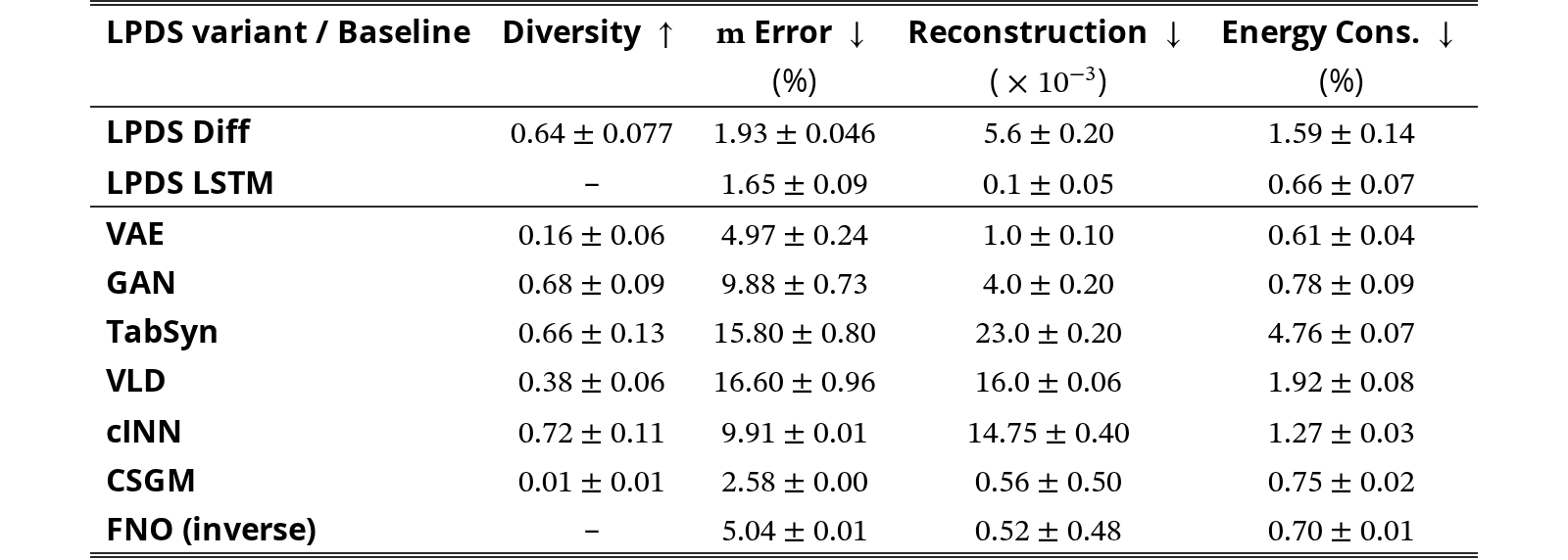
Table 7 highlights two failure modes that LPDS is designed to avoid. Amortized conditional generators trained without physics feedback (VAE, GAN, TabSyn, VLD, cINN, FNO) leave a large gap in outcome consistency, with errors between and , compared with for . In particular, the cINN, a flow-based approach of the kind used for neural posterior estimation, reaches high diversity but a error, illustrating the difficulty of scaling tractable-density posteriors to a 256-dimensional structured output. Conversely, test-time optimization against the surrogate (CSGM) attains a competitive error of only by collapsing diversity to , and must be rerun for every new . LPDS combines an expressive conditional generator with surrogate and physics feedback during training (, ), and is the only approach that combines an error below with high diversity, while keeping energy violation below .
We performed an ablation study by systematically varying the relative weights assigned to the reconstruction term () and the outcome-consistency term () in the composite loss 12, while keeping the physics penalty weight () constant. This analysis isolates the inherent trade-off surface between generating highly faithful, but potentially less diverse, laser pulse shapes (high ) and generating diverse solutions that effectively satisfy the target outcome (high ).
Figure 7 illustrates this critical trade-off. As the model’s objective shifts towards maximizing exploration of the design space (increasing ), it must tolerate a corresponding degradation in the reconstruction fidelity ().
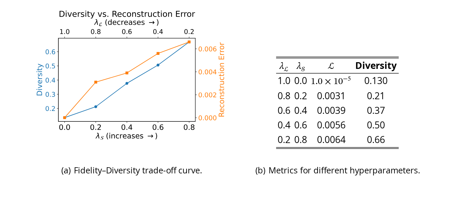
The results demonstrate a clear Pareto frontier. When and (strong emphasis on reconstruction), the model acts primarily as an autoencoder, achieving near-perfect fidelity () but minimal design diversity (). Conversely, as the weight shifts to strongly prioritize the surrogate outcome (), diversity reaches its maximum () at the expense of fidelity (). We excluded and because the model failed to learn physically viable representations.
This section evaluates the violation rates for the two primary operational constraints investigated: the instantaneous per-timestep maximum power caps and the maximum cumulative energy allowed during ICF experiments. These rates, detailed in Table 8, are crucial indicators of the robustness and feasibility of the generated LPs.
| Approach | Maximum Power Cap | Maximum Cumulative Energy |
|---|---|---|
| LSTM | 0 | 0 |
| Transformer | 0 | 0 |
| Diffusion | 0 | 0 |
| LSTM | 0 | 0 |
| LSTM | 0 | 0 |
| LSTM | 0 | 0 |
View original table
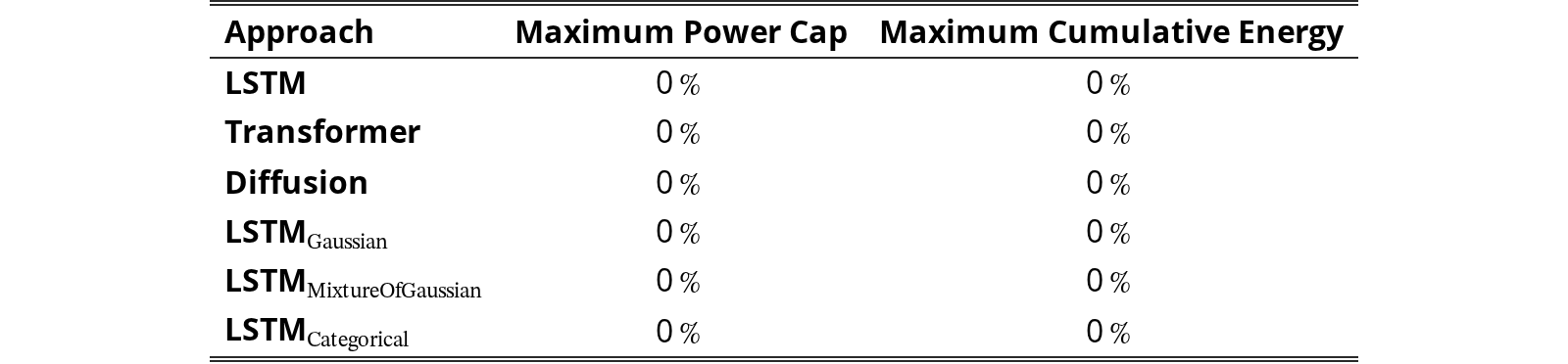
The data in Table 8 show that all approaches, including all LSTM variants (standard, Gaussian, mixture of Gaussians, and categorical), the Transformer, and the diffusion model, achieved 0% violation rates for both the instantaneous power cap and the cumulative energy constraint on this evaluation. This outcome indicates that and provide sufficient guidance during training for generation to remain within physically viable designs in the evaluated setting, without explicit constraint enforcement at inference time.
The random 70%–30% split used in the main experiments may place pulses from the same perturbation family in both the training and test sets. To evaluate generalization to genuinely unseen target designs, we construct a pellet-stratified split: we cluster the dataset with -means () on the pellet parameters and hold out the two clusters closest to the median cluster size, so that test pellet configurations are disjoint from those seen during training. Table 9 reports the error of on the held-out clusters. As a reference, we also report the error obtained by passing the ground-truth pulses of the held-out clusters through the surrogate, which gives the error floor attainable on these clusters.
| Setting | Error (%) |
|---|---|
| Random split, (Table 1) | 1.93 |
| Pellet-stratified split, ground-truth pulses (surrogate floor) | 1.53 |
| Pellet-stratified split, | 2.02 |
View original table

On the held-out pellet clusters, reaches a error, only percentage points above the surrogate floor and percentage points above its performance on the random split. This indicates that LPDS generalizes to unseen pellet configurations rather than interpolating within known perturbation families.
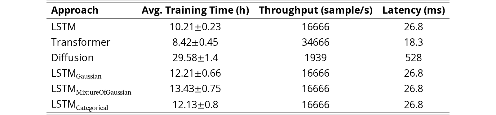
We analyze the computational overhead for training and inference (sampling) across the different approaches. While the training and inference costs are negligible when considering the month lead time and scale of the ICF experimental cycle, we study these properties because they are paramount for evaluating the model’s scalability and applicability to other scientific inverse design tasks where time-to-solution is a critical constraint. All reported times are based on the execution using a single NVIDIA H100 GPU for both training and inference tasks.
Table 10 presents the average training duration, samples generated per second and latency in milliseconds (time per batch). The training time is an average over 5 independent runs, with convergence defined as the point where the validation loss did not meaningfully improve over 20 consecutive epochs. The sampling time reports the average samples/time, when evaluated over the entire test set. These results highlight the intrinsic trade-offs among model complexity, training investment, and broader scientific utility.
| Approach | Avg. Training Time (h) | Throughput (sample/s) | Latency (ms) |
|---|---|---|---|
| LSTM | 10.210.23 | 16666 | 26.8 |
| Transformer | 8.420.45 | 34666 | 18.3 |
| Diffusion | 29.581.4 | 1939 | 528 |
| LSTM | 12.210.66 | 16666 | 26.8 |
| LSTM | 13.430.75 | 16666 | 26.8 |
| LSTM | 12.130.8 | 16666 | 26.8 |
View original table
The systematic benchmarking and ablation studies provide concrete, data-driven guidance for selecting the optimal generative strategy based on the specific goals of ICF LP generation. The decision-making process involves two stages: 1) selecting the appropriate generative architecture (Table 1), and 2) tuning the composite loss weights () to manage the Bias-Variance trade-off (Figure 7).
The choice of model is primarily dictated by the required balance between solution fidelity and design diversity(Table 1):
- •
Scenario 1: High Fidelity / Low Risk (Interpolation): If the goal is to generate LPs closely resembling known, successful designs from the training set (e.g., for marginal improvements or verification), models with low Reconstruction Error and low Error are preferred. The Deterministic LSTM network is ideal due to its high fidelity and strong Energy Conservation. These models act as robust interpolators but offer no novelty.
- •
Scenario 2: Balanced Exploration (Best Generalist): If the objective is to generate novel, diverse LPs while maintaining strong implosion performance, a probabilistic model is required. The Diffusion Model and LSTM offer the best trade-off. The Diffusion model offers superior diversity, while the LSTM is more physically consistent and computationally cheaper.
Once the architecture is chosen, the weights must be set based on the desired level of novelty versus realism. The ablation study in Figure 7 explicitly maps this trade-off:
- •
Conservative Setting (Minimize Variance): To minimize the risk of generating non-physical, low-fidelity LPs, one should set . This corresponds to the region of the Pareto curve where is lowest (e.g., , ). This strategy minimizes the solution variance but introduces strong bias toward the training distribution, limiting novelty.
- •
Exploratory Setting (Minimize Bias): To maximize the generation of novel LPs (minimizing bias against unexplored regions), one should accept a higher reconstruction loss. This corresponds to the highest diversity region (e.g., , Div ). This strategy maximizes novelty but increases the variance and risk of generating unstable pulses.
- •
Optimal Balance: For our application, the optimal choice lies at the middle of the Fidelity-Diversity Pareto frontier (e.g., ). This setting maximizes the gain in diversity (novelty) for the smallest corresponding cost in reconstruction fidelity (realism), offering the best overall stability and design utility.
Equation 12 defines the composite loss
where denotes the reconstruction or likelihood term, the outcome-consistency term using the differentiable surrogate , and the physics penalty. Because is a nonconvex objective, global optimality cannot be guaranteed. However, under standard smoothness and bounded-variance assumptions for stochastic gradients, stochastic gradient descent (SGD) with a suitable step-size schedule converges to a first-order stationary point in expectation. Formally, if is -Lipschitz and stochastic gradients satisfy , then with constant step size we obtain the standard rate . In practice, adaptive methods such as Adam used in our experiments empirically achieve similar convergence behavior. This statement clarifies that the optimization of Equation 12 yields approximate stationary points of the joint empirical objective.
Below we provide an analysis of how surrogate approximation error affects the surrogate-based outcome-consistency loss. This makes explicit the mechanisms by which a nonzero surrogate error can propagate through the inverse model.
Let be a generated pulse for condition , let
and define the pointwise surrogate error
The surrogate-based outcome-consistency term is
Noting we have the exact identity
Applying the reverse triangle inequality yields the simple bound
Thus, pointwise surrogate error translates directly into an additive bound on the surrogate-implied outcome error: the surrogate loss is a proxy for the true outcome error up to the pointwise surrogate deviation.
The primary risk of using a surrogate model () in the loss function is that the generator () may exploit the surrogate’s approximation error to satisfy the loss function without satisfying the true physical objective.
Conditional Bound: The generator minimizes the true LILAC residual provided that the surrogate pointwise approximation error, , remains uniformly small across the region of laser-pulse space explored by the generator. Using the bound from Section F.2, , the surrogate-implied outcome error and the true LILAC outcome error differ only up to the magnitude of the surrogate approximation error.
Adversarial Exploitation: This robustness can fail if the generator produces an LP, , that acts as an adversarial example for the surrogate. This occurs when lies in a region of the design space where the surrogate is inaccurate, so is large. In that case, the generator may achieve low surrogate error while the true LILAC error remains large, that is, . This constitutes exploitation of the surrogate and can produce a physically misleading design. The reconstruction loss and physics penalty help mitigate this failure mode by filtering implausible designs. This interpretation is consistent with the ablation results in Section E.1, where removing prevents the model from learning physically viable pulses.
The ICF LP inverse design problem is a classic example of an ill-posed inverse problem, meaning the solution is non-identifiable: multiple distinct LPs () can produce close fusion outcomes ().
Inverse Problem Constraint: Minimizing the outcome loss () alone would force the generator to converge to any LP that satisfies the desired outcome, likely producing an average or non-physical pulse shape located far from the actual manifold of feasible LPs (as described in Section E.1).
Regularization by : The Reconstruction Loss () is required to regularize the non-identifiable problem. By enforcing fidelity to the training data manifold, forces the generated solution to be the closest physically plausible pulse to the training set that also satisfies the outcome constraint. effectively selects a unique, stable solution from the infinite set of LPs that minimize .
The ablation study varying (Figure 7(b)) explicitly maps the bias–variance trade-off in the generated output:
Variance ( dominance): A low encourages the generator to explore further from the training manifold to satisfy the outcome, thus leading to high diversity and an increased variance.
Bias ( dominance): A high severely constrains the generator to the known training data, leading to low diversity (low variance). This strategy is robust but prone to bias against novel pulse shapes that may lie slightly outside the training data distribution.
A key concern when employing surrogate models is whether their approximation error remains stable when the generator produces pulses that differ from those seen during surrogate training. To quantify this effect, we compare the implosion-outcome error for generated pulses with a simple novelty measure computed relative to the original training dataset.
Given a generated pulse , we define its novelty as its distance to the closest pulse in the training set :
This quantity measures how far the generator has moved away from the region where the surrogate has been trained and validated, and therefore acts as a proxy for out-of-distribution (OOD) deviation.
We compute the surrogate outcome-consistency error
The magnitude reflects the squared surrogate residual induced by . This is the same quantity used inside the loss in Equation 10; unlike the main-text evaluation metric, it is not reported as MAPE.
To assess whether systematically increases as pulses move farther from the training manifold, we compute the Spearman rank correlation
Spearman correlation is insensitive to scale and captures monotonic relationships, making it appropriate for detecting trends such as “greater novelty larger surrogate error.” A strong positive correlation would indicate that introduces a strong bias in the generative model against OOD regions, while a correlation close to zero would suggest that the surrogate maintains relatively uniform influence across the generator’s operating domain.
We ran this evaluation using Diffusion as the base model since it offers a good balance between error and diversity. The Spearman correlation between implosion-outcome error magnitude and the novelty score on the test set is with . This modest correlation indicates that the surrogate error exhibits a mild monotonic increase with distance from the training manifold. The effect size is not strong, suggesting that the surrogate remains reasonably reliable across the region of pulse space that the generative models operate in. Importantly, this behavior is consistent with expectations for neural surrogates trained on physically coherent waveform datasets: their accuracy degrades smoothly with novelty but does not break down or dramatically inflate in regions relevant to our experiments.
Moreover, as shown by the diffusion model results, diversity does not negatively affect , since the model achieves high diversity while maintaining low error.
The correlation above shows that surrogate error grows only mildly with novelty; we further check how far generated pulses actually move from the training data. We compute the novelty score for three populations: training pulses (distance to their nearest other training pulse, ), test pulses (), and pulses generated by for one of the held-out pellet clusters of Appendix E.3 (). Table 11 reports the mean novelty of each population and the fraction of samples beyond the 95th percentile of the test-set novelty distribution.
| Population | Mean novelty | 95th percentile | Fraction beyond test 95th percentile |
|---|---|---|---|
| Training (nearest other training pulse) | 0.7125 | 1.0807 | – |
| Test | 0.7125 | 1.0814 | 5.00% |
| (held-out pellet cluster) | 0.7048 | – | 5.04% |
View original table

Generated pulses are, on average, slightly closer to the training data than held-out test pulses ( vs. ), and the fraction beyond the test 95th percentile () matches the expected for in-distribution samples. Together with the mild correlation reported above, this indicates that neither drifts away from the training manifold nor relies on off-manifold regions where the surrogate is unreliable.
To enhance controllability during generation, LPDS supports inpainting as a mechanism for partial conditioning directly in the laser pulse space. This allows domain experts to specify only certain segments of a laser pulse, while leaving the remaining parts to be completed by the model in a physically consistent manner.
Formally, let denote a laser pulse of length , and let be a binary mask that defines the constraint region. Each element indicates whether the -th component of the pulse is observed () or masked (). Let represent the observed (non-masked) entries of the pulse.
To incorporate inpainting with Diffusion, we modify the reverse diffusion process so that known regions remain fixed at each step. Let be the predicted intermediate pulse at timestep from the standard DDIM update rule (Equation 4). We define the inpainted latent state as:
where denotes elementwise multiplication. This formulation ensures that the observed parts of the pulse are preserved throughout the denoising process, while the model only modifies the masked (unknown) components.
In practice, the mask can be flexibly defined to support a wide range of expert interactions, for example, preserving a fixed peak intensity, pre-specified rising edge, or constraints learned from past experiments. Combined with the implosion outcomes and target parameters conditioning via and , inpainting enables LPDS to support fine-grained, interpretable, and editable pulse design.
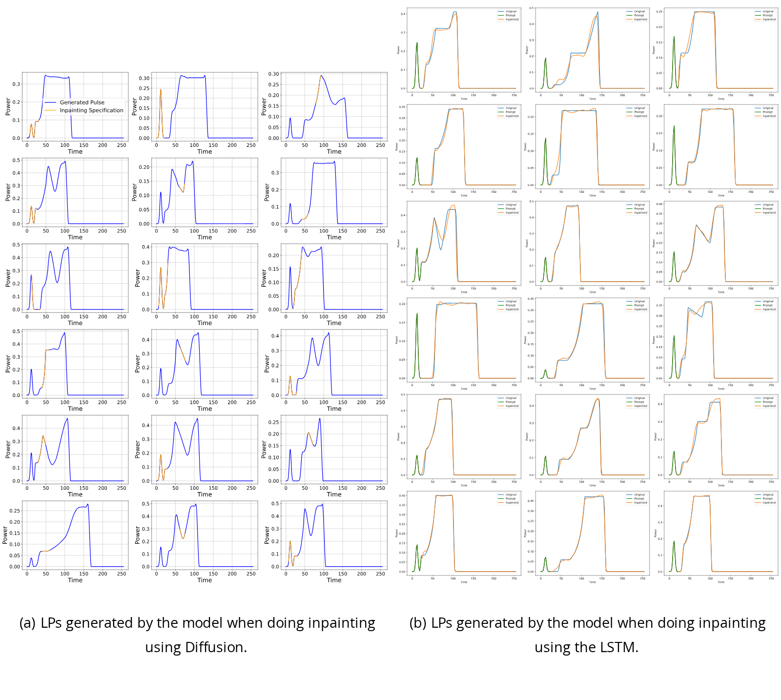
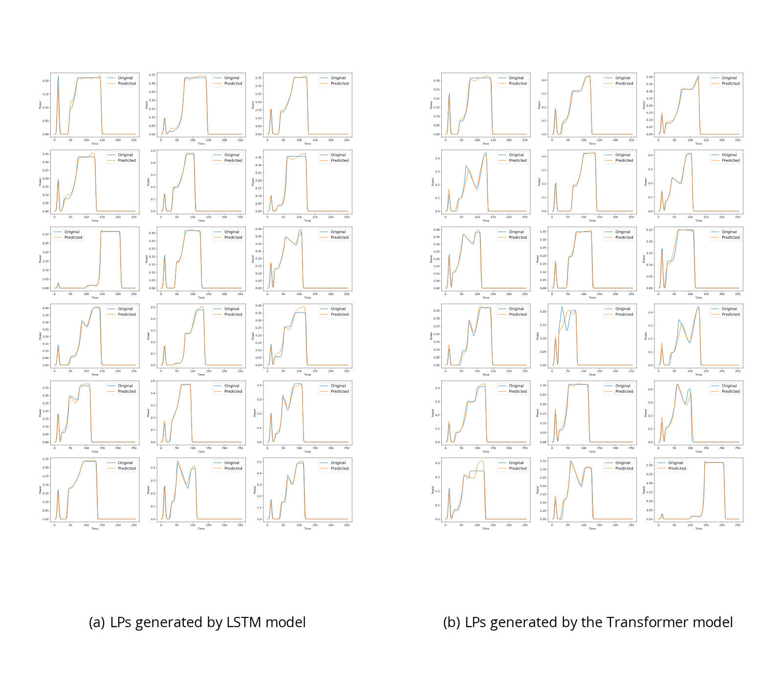
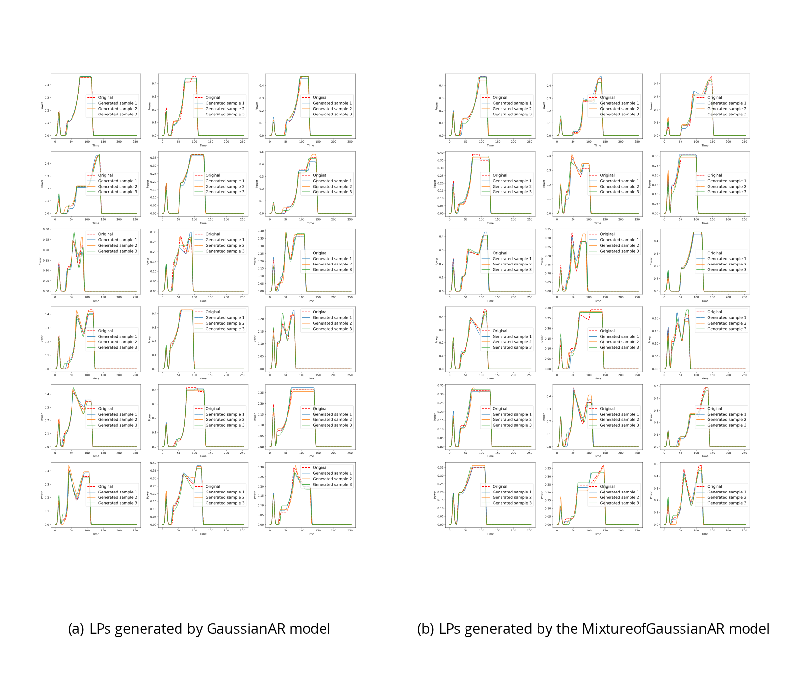
We present some of the pulses generated by the different approaches. Figure 9(b) for Diffusion, Figure 10(a) for LSTM, Figure 10(b) for Transformer, Figure 11(a) for GaussianAR, Figure 11(b) for MixtureOfGaussianAR. Figure 12 shows examples of LPs generated by the LP novel design method described in Section 5.5
This work aims to accelerate inverse design for inertial confinement fusion, which could contribute positively to scientific discovery in high-energy-density physics and, in the long term, to cleaner energy technologies if fusion becomes practical. More broadly, the methodological contributions may also benefit other scientific inverse-design problems where multiple physically plausible solutions must be generated under hard constraints.
Potential negative impacts are primarily indirect. Improved inverse-design and optimization tools could be misapplied to accelerate the design of high-energy systems beyond the intended scientific context.
- 1.
Claims
Question: Do the main claims made in the abstract and introduction accurately reflect the paper’s contributions and scope?
Answer: [Yes]
Justification: Yes. The abstract and introduction state the main claims about LPDS, its controllable generation mechanisms, and simulator-grounded validation, and these claims are supported by the experimental and theoretical sections.
Guidelines:
- •
The answer [N/A] means that the abstract and introduction do not include the claims made in the paper.
- •
The abstract and/or introduction should clearly state the claims made, including the contributions made in the paper and important assumptions and limitations. A [No] or [N/A] answer to this question will not be perceived well by the reviewers.
- •
The claims made should match theoretical and experimental results, and reflect how much the results can be expected to generalize to other settings.
- •
It is fine to include aspirational goals as motivation as long as it is clear that these goals are not attained by the paper.
- •
- 2.
Limitations
Question: Does the paper discuss the limitations of the work performed by the authors?
Answer: [Yes]
Justification: Yes. The paper includes a dedicated Limitations section discussing regime.
Guidelines:
- •
The answer [N/A] means that the paper has no limitation while the answer [No] means that the paper has limitations, but those are not discussed in the paper.
- •
The authors are encouraged to create a separate “Limitations” section in their paper.
- •
The paper should point out any strong assumptions and how robust the results are to violations of these assumptions (e.g., independence assumptions, noiseless settings, model well-specification, asymptotic approximations only holding locally). The authors should reflect on how these assumptions might be violated in practice and what the implications would be.
- •
The authors should reflect on the scope of the claims made, e.g., if the approach was only tested on a few datasets or with a few runs. In general, empirical results often depend on implicit assumptions, which should be articulated.
- •
The authors should reflect on the factors that influence the performance of the approach. For example, a facial recognition algorithm may perform poorly when image resolution is low or images are taken in low lighting. Or a speech-to-text system might not be used reliably to provide closed captions for online lectures because it fails to handle technical jargon.
- •
The authors should discuss the computational efficiency of the proposed algorithms and how they scale with dataset size.
- •
If applicable, the authors should discuss possible limitations of their approach to address problems of privacy and fairness.
- •
While the authors might fear that complete honesty about limitations might be used by reviewers as grounds for rejection, a worse outcome might be that reviewers discover limitations that aren’t acknowledged in the paper. The authors should use their best judgment and recognize that individual actions in favor of transparency play an important role in developing norms that preserve the integrity of the community. Reviewers will be specifically instructed to not penalize honesty concerning limitations.
- •
- 3.
Theory assumptions and proofs
Question: For each theoretical result, does the paper provide the full set of assumptions and a complete (and correct) proof?
Answer: [N/A]
Justification: The paper does not include theoretical results
Guidelines:
- •
The answer [N/A] means that the paper does not include theoretical results.
- •
All the theorems, formulas, and proofs in the paper should be numbered and cross-referenced.
- •
All assumptions should be clearly stated or referenced in the statement of any theorems.
- •
The proofs can either appear in the main paper or the supplemental material, but if they appear in the supplemental material, the authors are encouraged to provide a short proof sketch to provide intuition.
- •
Inversely, any informal proof provided in the core of the paper should be complemented by formal proofs provided in appendix or supplemental material.
- •
Theorems and Lemmas that the proof relies upon should be properly referenced.
- •
- 4.
Experimental result reproducibility
Question: Does the paper fully disclose all the information needed to reproduce the main experimental results of the paper to the extent that it affects the main claims and/or conclusions of the paper (regardless of whether the code and data are provided or not)?
Answer: [Yes]
Justification: Yes. The paper specifies the dataset construction, evaluation metrics, number of runs and seeds, train/test splits, hyperparameter search ranges, optimizer choices, and compute setup in the main paper and appendix Experimental Details.
Guidelines:
- •
The answer [N/A] means that the paper does not include experiments.
- •
If the paper includes experiments, a [No] answer to this question will not be perceived well by the reviewers: Making the paper reproducible is important, regardless of whether the code and data are provided or not.
- •
If the contribution is a dataset and/or model, the authors should describe the steps taken to make their results reproducible or verifiable.
- •
Depending on the contribution, reproducibility can be accomplished in various ways. For example, if the contribution is a novel architecture, describing the architecture fully might suffice, or if the contribution is a specific model and empirical evaluation, it may be necessary to either make it possible for others to replicate the model with the same dataset, or provide access to the model. In general. releasing code and data is often one good way to accomplish this, but reproducibility can also be provided via detailed instructions for how to replicate the results, access to a hosted model (e.g., in the case of a large language model), releasing of a model checkpoint, or other means that are appropriate to the research performed.
- •
While NeurIPS does not require releasing code, the conference does require all submissions to provide some reasonable avenue for reproducibility, which may depend on the nature of the contribution. For example
- (a)
If the contribution is primarily a new algorithm, the paper should make it clear how to reproduce that algorithm.
- (b)
If the contribution is primarily a new model architecture, the paper should describe the architecture clearly and fully.
- (c)
If the contribution is a new model (e.g., a large language model), then there should either be a way to access this model for reproducing the results or a way to reproduce the model (e.g., with an open-source dataset or instructions for how to construct the dataset).
- (d)
We recognize that reproducibility may be tricky in some cases, in which case authors are welcome to describe the particular way they provide for reproducibility. In the case of closed-source models, it may be that access to the model is limited in some way (e.g., to registered users), but it should be possible for other researchers to have some path to reproducing or verifying the results.
- (a)
- •
- 5.
Open access to data and code
Question: Does the paper provide open access to the data and code, with sufficient instructions to faithfully reproduce the main experimental results, as described in supplemental material?
Answer: [No]
Justification: We will release the code upon publication.
Guidelines:
- •
The answer [N/A] means that paper does not include experiments requiring code.
- •
Please see the NeurIPS code and data submission guidelines (https://neurips.cc/public/guides/CodeSubmissionPolicy) for more details.
- •
While we encourage the release of code and data, we understand that this might not be possible, so [No] is an acceptable answer. Papers cannot be rejected simply for not including code, unless this is central to the contribution (e.g., for a new open-source benchmark).
- •
The instructions should contain the exact command and environment needed to run to reproduce the results. See the NeurIPS code and data submission guidelines (https://neurips.cc/public/guides/CodeSubmissionPolicy) for more details.
- •
The authors should provide instructions on data access and preparation, including how to access the raw data, preprocessed data, intermediate data, and generated data, etc.
- •
The authors should provide scripts to reproduce all experimental results for the new proposed method and baselines. If only a subset of experiments are reproducible, they should state which ones are omitted from the script and why.
- •
At submission time, to preserve anonymity, the authors should release anonymized versions (if applicable).
- •
Providing as much information as possible in supplemental material (appended to the paper) is recommended, but including URLs to data and code is permitted.
- •
- 6.
Experimental setting/details
Question: Does the paper specify all the training and test details (e.g., data splits, hyperparameters, how they were chosen, type of optimizer) necessary to understand the results?
Answer: [Yes]
Justification: Yes. The paper and appendix specify the data split, training setup, hyperparameter ranges, selected hyperparameters, optimizer, scheduler, and model-specific settings needed to understand the experiments.
Guidelines:
- •
The answer [N/A] means that the paper does not include experiments.
- •
The experimental setting should be presented in the core of the paper to a level of detail that is necessary to appreciate the results and make sense of them.
- •
The full details can be provided either with the code, in appendix, or as supplemental material.
- •
- 7.
Experiment statistical significance
Question: Does the paper report error bars suitably and correctly defined or other appropriate information about the statistical significance of the experiments?
Answer: [Yes]
Justification: Yes. The main result tables report variability with values.
Guidelines:
- •
The answer [N/A] means that the paper does not include experiments.
- •
The authors should answer [Yes] if the results are accompanied by error bars, confidence intervals, or statistical significance tests, at least for the experiments that support the main claims of the paper.
- •
The factors of variability that the error bars are capturing should be clearly stated (for example, train/test split, initialization, random drawing of some parameter, or overall run with given experimental conditions).
- •
The method for calculating the error bars should be explained (closed form formula, call to a library function, bootstrap, etc.)
- •
The assumptions made should be given (e.g., Normally distributed errors).
- •
It should be clear whether the error bar is the standard deviation or the standard error of the mean.
- •
It is OK to report 1-sigma error bars, but one should state it. The authors should preferably report a 2-sigma error bar than state that they have a 96% CI, if the hypothesis of Normality of errors is not verified.
- •
For asymmetric distributions, the authors should be careful not to show in tables or figures symmetric error bars that would yield results that are out of range (e.g., negative error rates).
- •
If error bars are reported in tables or plots, the authors should explain in the text how they were calculated and reference the corresponding figures or tables in the text.
- •
- 8.
Experiments compute resources
Question: For each experiment, does the paper provide sufficient information on the computer resources (type of compute workers, memory, time of execution) needed to reproduce the experiments?
Answer: [Yes]
Justification: Yes. The appendix reports the hardware used, total project-scale compute, single-GPU timing assumptions, average training times, throughput, and latency measurements for the main approaches.
Guidelines:
- •
The answer [N/A] means that the paper does not include experiments.
- •
The paper should indicate the type of compute workers CPU or GPU, internal cluster, or cloud provider, including relevant memory and storage.
- •
The paper should provide the amount of compute required for each of the individual experimental runs as well as estimate the total compute.
- •
The paper should disclose whether the full research project required more compute than the experiments reported in the paper (e.g., preliminary or failed experiments that didn’t make it into the paper).
- •
- 9.
Code of ethics
Question: Does the research conducted in the paper conform, in every respect, with the NeurIPS Code of Ethics https://neurips.cc/public/EthicsGuidelines?
Answer: [Yes]
Justification: Yes. To the best of our knowledge, the research described in the paper conforms to the NeurIPS Code of Ethics.
Guidelines:
- •
The answer [N/A] means that the authors have not reviewed the NeurIPS Code of Ethics.
- •
If the authors answer [No] , they should explain the special circumstances that require a deviation from the Code of Ethics.
- •
The authors should make sure to preserve anonymity (e.g., if there is a special consideration due to laws or regulations in their jurisdiction).
- •
- 10.
Broader impacts
Question: Does the paper discuss both potential positive societal impacts and negative societal impacts of the work performed?
Answer: [Yes]
Justification: Yes. The appendix now includes a dedicated Broader Impacts section discussing potential positive scientific and energy-related benefits as well as possible misuse risks.
Guidelines:
- •
The answer [N/A] means that there is no societal impact of the work performed.
- •
If the authors answer [N/A] or [No] , they should explain why their work has no societal impact or why the paper does not address societal impact.
- •
Examples of negative societal impacts include potential malicious or unintended uses (e.g., disinformation, generating fake profiles, surveillance), fairness considerations (e.g., deployment of technologies that could make decisions that unfairly impact specific groups), privacy considerations, and security considerations.
- •
The conference expects that many papers will be foundational research and not tied to particular applications, let alone deployments. However, if there is a direct path to any negative applications, the authors should point it out. For example, it is legitimate to point out that an improvement in the quality of generative models could be used to generate Deepfakes for disinformation. On the other hand, it is not needed to point out that a generic algorithm for optimizing neural networks could enable people to train models that generate Deepfakes faster.
- •
The authors should consider possible harms that could arise when the technology is being used as intended and functioning correctly, harms that could arise when the technology is being used as intended but gives incorrect results, and harms following from (intentional or unintentional) misuse of the technology.
- •
If there are negative societal impacts, the authors could also discuss possible mitigation strategies (e.g., gated release of models, providing defenses in addition to attacks, mechanisms for monitoring misuse, mechanisms to monitor how a system learns from feedback over time, improving the efficiency and accessibility of ML).
- •
- 11.
Safeguards
Question: Does the paper describe safeguards that have been put in place for responsible release of data or models that have a high risk for misuse (e.g., pre-trained language models, image generators, or scraped datasets)?
Answer: [N/A]
Justification: The paper does not release high-risk generative models or scraped datasets.
Guidelines:
- •
The answer [N/A] means that the paper poses no such risks.
- •
Released models that have a high risk for misuse or dual-use should be released with necessary safeguards to allow for controlled use of the model, for example by requiring that users adhere to usage guidelines or restrictions to access the model or implementing safety filters.
- •
Datasets that have been scraped from the Internet could pose safety risks. The authors should describe how they avoided releasing unsafe images.
- •
We recognize that providing effective safeguards is challenging, and many papers do not require this, but we encourage authors to take this into account and make a best faith effort.
- •
- 12.
Licenses for existing assets
Question: Are the creators or original owners of assets (e.g., code, data, models), used in the paper, properly credited and are the license and terms of use explicitly mentioned and properly respected?
Answer: [N/A]
Justification: We do not use existing assets.
Guidelines:
- •
The answer [N/A] means that the paper does not use existing assets.
- •
The authors should cite the original paper that produced the code package or dataset.
- •
The authors should state which version of the asset is used and, if possible, include a URL.
- •
The name of the license (e.g., CC-BY 4.0) should be included for each asset.
- •
For scraped data from a particular source (e.g., website), the copyright and terms of service of that source should be provided.
- •
If assets are released, the license, copyright information, and terms of use in the package should be provided. For popular datasets, paperswithcode.com/datasets has curated licenses for some datasets. Their licensing guide can help determine the license of a dataset.
- •
For existing datasets that are re-packaged, both the original license and the license of the derived asset (if it has changed) should be provided.
- •
If this information is not available online, the authors are encouraged to reach out to the asset’s creators.
- •
- 13.
New assets
Question: Are new assets introduced in the paper well documented and is the documentation provided alongside the assets?
Answer: [N/A]
Justification: The paper does not release new assets.
Guidelines:
- •
The answer [N/A] means that the paper does not release new assets.
- •
Researchers should communicate the details of the dataset/code/model as part of their submissions via structured templates. This includes details about training, license, limitations, etc.
- •
The paper should discuss whether and how consent was obtained from people whose asset is used.
- •
At submission time, remember to anonymize your assets (if applicable). You can either create an anonymized URL or include an anonymized zip file.
- •
- 14.
Crowdsourcing and research with human subjects
Question: For crowdsourcing experiments and research with human subjects, does the paper include the full text of instructions given to participants and screenshots, if applicable, as well as details about compensation (if any)?
Answer: [N/A]
Justification: The work does not involve crowdsourcing or research with human subjects.
Guidelines:
- •
The answer [N/A] means that the paper does not involve crowdsourcing nor research with human subjects.
- •
Including this information in the supplemental material is fine, but if the main contribution of the paper involves human subjects, then as much detail as possible should be included in the main paper.
- •
According to the NeurIPS Code of Ethics, workers involved in data collection, curation, or other labor should be paid at least the minimum wage in the country of the data collector.
- •
- 15.
Institutional review board (IRB) approvals or equivalent for research with human subjects
Question: Does the paper describe potential risks incurred by study participants, whether such risks were disclosed to the subjects, and whether Institutional Review Board (IRB) approvals (or an equivalent approval/review based on the requirements of your country or institution) were obtained?
Answer: [N/A]
Justification: The work does not involve crowdsourcing or research with human subjects.
Guidelines:
- •
The answer [N/A] means that the paper does not involve crowdsourcing nor research with human subjects.
- •
Depending on the country in which research is conducted, IRB approval (or equivalent) may be required for any human subjects research. If you obtained IRB approval, you should clearly state this in the paper.
- •
We recognize that the procedures for this may vary significantly between institutions and locations, and we expect authors to adhere to the NeurIPS Code of Ethics and the guidelines for their institution.
- •
For initial submissions, do not include any information that would break anonymity (if applicable), such as the institution conducting the review.
- •
- 16.
Declaration of LLM usage
Question: Does the paper describe the usage of LLMs if it is an important, original, or non-standard component of the core methods in this research? Note that if the LLM is used only for writing, editing, or formatting purposes and does not impact the core methodology, scientific rigor, or originality of the research, declaration is not required.
Answer: [N/A]
Justification: The core method does not use LLMs as an important, original, or non-standard methodological component.
Guidelines:
- •
The answer [N/A] means that the core method development in this research does not involve LLMs as any important, original, or non-standard components.
- •
Please refer to our LLM policy in the NeurIPS handbook for what should or should not be described.
- •