Contrastive Discovery: Open-Ended Scientific Discovery over Competing Explanations
arXiv:2611.14514v1 · This workspace stays on this version. Check arXiv for newer versions
Some source details need review 2 to check
Original formulas, table values and figures are preserved. Comparison can miss differences; use the original PDF to check details.
Reading view checked: 496 math expressions, 0 rendering failures; 28 of 28 images available.
Compared 146 of 221 source passages against 28 of 55 PDF pages.
- This long paper was only partially compared; the original sources remain available.
HTML S3_SS5_p2_1 reads “details in Appendix ;”, while the original PDF page 5 visibly reads “details in Appendix T.1;”. The PDF includes the omitted reference. Check PDF page 5
28 of 28 figure, table and graphic images captured. Open original PDF
Abstract
LLM agents are increasingly used for open-ended, data-driven scientific discovery, yet most of them evaluate hypotheses pointwise, testing an empirical claim only against its complement . When evidence rejects , the agent learns that one explanation is unlikely but not which alternative the evidence supports. To recover that alternative, we introduce Contrastive Discovery, which replaces the single hypothesis with a contrast set, a scientific question paired with mutually exclusive and collectively exhaustive competing explanations. Each experiment is scored by how its evidence redistributes belief across the set, and the question is resolved when belief concentrates on one explanation. Because contrast sets change only the unit an agent proposes and scores, an existing agent can use them to re-evaluate evidence it has already collected or to guide its search. Across six domains, 89% of the pointwise candidates with the largest belief shifts are rejections. On the same evidence, contrast sets resolve 73% of these candidates to a specific alternative. When contrast sets guide search, the agent resolves 67% more questions than pointwise surprisal under the same experiment budget. In a blinded study, 38 human experts chose the same explanation on 78% of resolved questions and on 82% of questions where the pointwise agent rejected its hypothesis and stopped. Together, these results support explicit competing explanations as a way for discovery agents to resolve more scientific questions from the same evidence and validation budget.
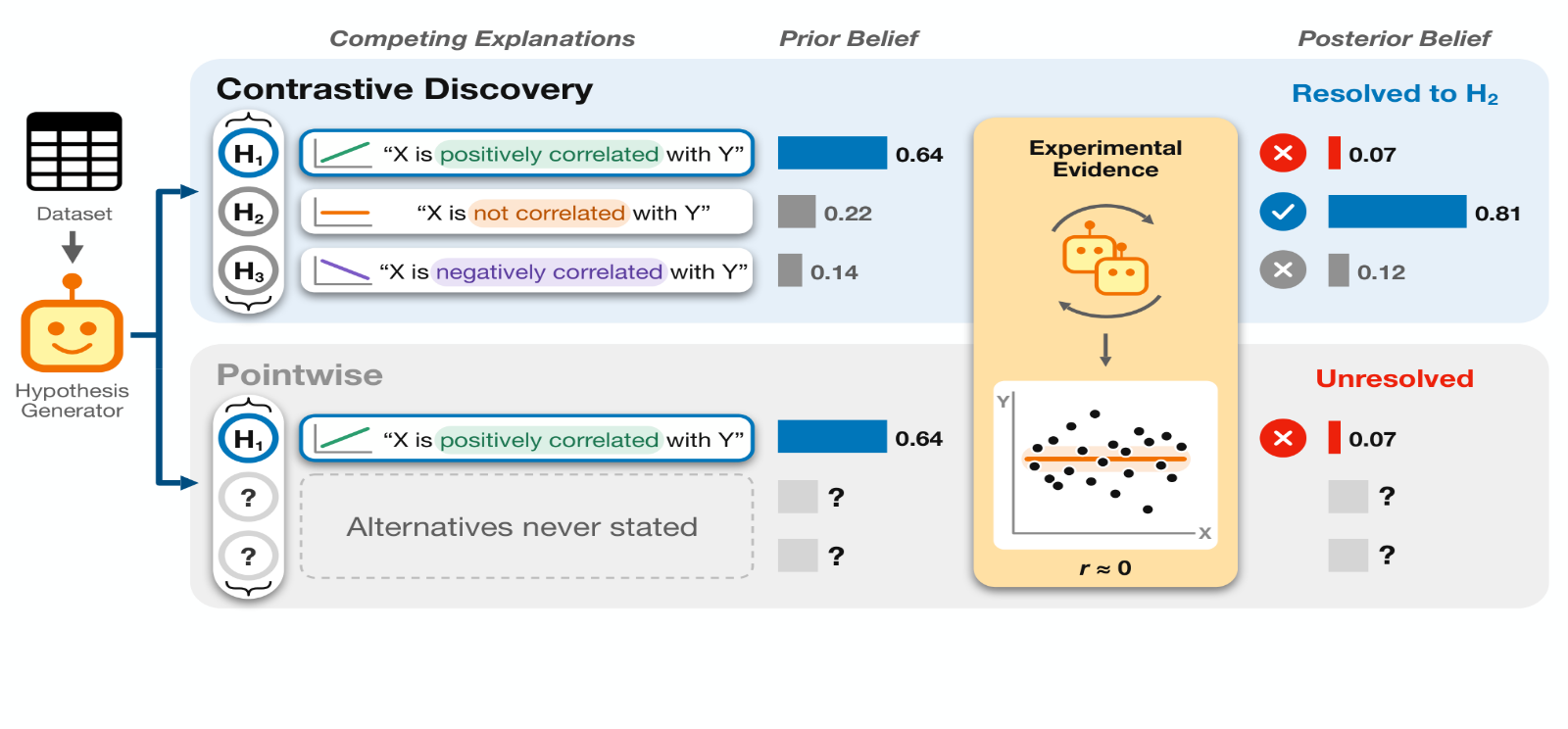
The shift toward autonomous scientific discovery has been accelerated by agents that generate hypotheses, design experiments, collect evidence, and iterate on candidate findings [29, 43, 19, 35]. Recent systems scale this loop to evaluate hundreds or thousands of discoveries across scientific domains [2, 11, 17]. At this scale, measuring progress becomes a problem. In closed tasks, progress is measured against fixed objectives, answer keys, or benchmarks [33, 45], but open-ended discovery has no oracle specifying which discovery should come next. Without an oracle, progress depends not only on how each candidate is scored, but on what unit of knowledge the agent treats as learned.
In most current discovery systems, that unit is a single hypothesis. The agent proposes an empirical claim , tests it, scores the result, and then keeps, revises, or discards [13, 31, 11]. The score may be an LLM judgment of novelty or feasibility [4, 10, 24, 34], or a belief-shift objective such as Bayesian surprise [2, 18], which treats discovery as evidence-induced belief change rather than a subjective judgment of interestingness. Yet the representational unit of progress stays the same: evidence updates belief in one focal hypothesis against its implicit complement . We call this pointwise discovery. This formulation is shared across agentic discovery systems that otherwise differ in how they propose hypotheses, gather evidence, and score discoveries.
The pointwise representation is epistemically limiting because scientific evidence often discriminates among plausible alternatives rather than supporting a single hypothesis in isolation. This limitation is clearest when evidence rejects a proposed hypothesis : the agent learns that the focal hypothesis is unlikely, but not which alternative is better supported. For example, evidence against “self-employed applicants with poor credit face higher mortgage denial rates” does not say whether their denial rates are lower or no different. Under a fixed evidence-generation budget, this is information-inefficient: the agent may need additional hypothesis proposals and evaluations to resolve a scientific question that the original evidence already helps answer.
We argue that open-ended discovery requires a larger unit of progress: a scientific question together with the plausible explanations that could answer it. This follows contrastive accounts of scientific explanation, in which evidence is informative because it discriminates among alternatives [41, 26]. We introduce Contrastive Discovery, which represents each discovery step as a contrast set (Eq. 1, Figure 1): a set of mutually exclusive and collectively exhaustive (MECE) explanations answering one question. The agent elicits prior and posterior beliefs over the set and scores a candidate discovery by how much its evidence redistributes belief. A question is resolved when posterior belief concentrates on one explanation, so a single experiment can both rule out alternatives and identify the best-supported one. Otherwise, the evidence remains informative but the question is unresolved.
Contrast sets change the unit an agent proposes and scores, not its architecture, so they can be layered onto an existing agent in two ways. As an evaluation lens, they re-evaluate evidence the agent has already collected, without modifying the agent. To guide search, they replace the agent’s hypothesis and score, so the search is rewarded for evidence that discriminates among competing explanations. We evaluate Contrastive Discovery across six domains spanning materials science, astronomy, mortgage discrimination, online discourse, software engineering practices, and social behavior. Under a shared scaffold and evidence-generation budget, pointwise baselines are guided by surprisal, novelty, or feasibility, while Contrastive Discovery is guided by belief shift over contrast sets. We find:
- •
Pointwise rejections conceal resolvable alternatives. Across three elicitor models, a majority of pointwise proposals receive a “maybe true” prior, and 89% of the highest-surprisal pointwise candidates are rejections. Used as an evaluation lens on the same evidence, contrast sets resolve 73% of these candidates to a specific alternative without running new experiments (§5.1).
- •
Contrastive Discovery turns rejections into resolved questions. Guiding search with contrast sets resolves 67% more questions than pointwise surprisal under the same experiment budget. Nearly all the gain comes from corrective resolutions, where evidence shifts support away from the explanation favored beforehand; pointwise discovery records these cases only as rejections (§5.2).
- •
The gain comes from explicit alternatives and holds up under validation. Ablations trace the gain primarily to evaluating evidence against the full contrast set (§5.3). In a blinded study, 38 human experts chose the same explanation on 78% of resolved questions and on 82% where the pointwise agent rejected its hypothesis and stopped (§5.4). The gain holds when each alternative is scored independently with the pointwise scorer and at matched token and dollar cost (§5.5).
Discovery loop. We study open-ended, data-driven scientific discovery, where an agent uses a dataset to propose hypotheses , evaluates them using evidence computed from the data, and scores them, repeating under a budget of steps. The setting is open-ended because no predefined reward function determines the value of a discovery, which depends instead on the scientific question, the available evidence, and prior knowledge. This formulation captures recent LLM-based discovery systems [2].
Pointwise discovery. We call a discovery method pointwise when, at step , the agent proposes a single hypothesis and independently assesses it by scoring only that proposed candidate and its evidence. Many recent LLM-based discovery approaches are pointwise, assessing each hypothesis through novelty and feasibility [4, 10, 24], evidential support [11, 17], or Bayesian surprise [2]. In our notation (§3.5), pointwise discovery is the binary case of Contrastive Discovery, where the only alternative to is its negation.
The rejection case. In pointwise discovery, confirmation and rejection have different epistemic consequences. Confirmation identifies a supported explanation, but rejection only rules against the proposed one. The evidence may bear on alternatives, yet the pointwise score exposes only its effect on . Resolving among competing explanations then takes a separate step for each alternative, each drawn from the finite budget of steps, even when one experiment’s evidence bears on all of them.
We reframe a discovery step from validating a single candidate hypothesis to resolving a scientific question. We keep the evidence-induced belief-shift principle of surprisal-based discovery [2, 18] but change the unit over which belief is represented, from one hypothesis to a structured set of plausible explanations for the same question. The alternatives thereby become part of the unit, so they determine what the evidence is compared against, how belief is updated, and what outcome the step can produce.
At each discovery step , the agent poses a local scientific question and constructs a contrast set
where each is a plausible explanation for the same question. We require these explanations to be locally mutually exclusive and collectively exhaustive (MECE): within the scope of the question, no two of them can hold at once, and together they cover the main outcomes the evidence is meant to distinguish. For example, for the scientific question “Given a poor credit score, how is self-employment associated with mortgage denial rates?”, the three explanations in the contrast set are that self-employed applicants face higher, no different, or lower denial rates than other applicants (further examples in Appendix ).
Given a contrast set , we next define the belief state used to score evidence-induced change. Before observing evidence, we elicit where is the probability simplex over the explanations and is the subjective belief assigned to explanation . After the agent runs its experiment and observes evidence , we elicit . We treat these elicited distributions as the prior and posterior beliefs over the contrast set.
Computing the posterior by Bayes’ rule would require a hand-specified likelihood model for every analysis. We therefore obtain each distribution directly through a constant-sum allocation task: a belief elicitor, an LLM separate from the agent (§4), assigns 100 allocation units across the explanations in , first without and then with access to . To reduce stochastic variance, we sample five allocations and average the normalized valid responses (see Appendices and B). We also randomize the order of explanations during elicitation to mitigate positional bias in LLM-based evaluation (see Appendix D).
Because the unit of discovery is a belief distribution over competing explanations, the score should measure how evidence changes that distribution. Given prior and posterior beliefs and , we compute the Kullback–Leibler divergence () of with respect to . This direction is the Bayesian surprise of Itti and Baldi 18, the realized information gain from observing . The divergence tends to grow with the size of the contrast set, reaching bits when a uniform prior collapses onto one explanation, so we divide by to compare sets of different sizes. We call the result the contrastive belief shift, an entropy-scaled Bayesian surprise:
We use as the Contrastive Discovery score, and larger values mean that the evidence moved more belief across the competing explanations. Scaling does not bound by one, because evidence can move belief onto an explanation the prior considered unlikely. When we use as the tree-search reward (§4), we therefore clip it at one, , and all reported information-gain analyses use the unclipped (see Appendix ).
The contrastive belief shift measures the magnitude of belief shift, but not the type of discovery produced by that shift. Since the prior and posterior are defined over the same competing explanations, the update can also be characterized by whether evidence confirms the prior-leading explanation, shifts support to another explanation, rules out alternatives, or leaves the question unresolved. Let
denote the indices of the prior- and posterior-leading explanations. We say the question is resolved when the posterior assigns sufficient support to one explanation,
where is the minimum posterior support required to identify a leading explanation (we use and vary it in §5.5). A resolved update is confirmative if and corrective if , that is, when evidence moves support from the prior-leading explanation to another one. If no explanation reaches , the outcome is unresolved. A generated contrast set may omit the explanation the evidence supports. As a safeguard, we optionally add an abstention alternative, “none of the listed alternatives matches the evidence.” If its belief reaches , we flag a possible omission and report no resolution. The main experiments do not include this safeguard, and §5.4 tests it.
We separately track explanations that are ruled out: an explanation is ruled out when , where denotes a low posterior-support threshold (we use ). Ruling out is tracked apart from the three outcomes above, because a single contrastive update can identify a leading explanation and also rule out competing explanations. For the pointwise setting, where a single hypothesis has scalar prior and posterior beliefs, we classify the update analogously: a hypothesis is confirmed if its posterior reaches , rejected if it is at most , and ambiguous otherwise (we use and , with calibration details in Appendix E). The taxonomy thus separates how much support for a hypothesis rises or falls, which pointwise discovery captures, from which explanation the evidence favors, which requires explicit alternatives.
Pointwise belief-shift methods score evidence by how much it changes belief in a single hypothesis . In our notation, this is the binary contrast set with belief state , where is belief in and is belief in its complement. In this representation, pointwise discovery is the instance of Contrastive Discovery, where the only alternative contains all ways the focal hypothesis could be false. Thus, when evidence weakens , pointwise discovery can record negative evidence about the claim but cannot identify which alternative explanation receives that support. Contrastive Discovery replaces this complement with an explicit local partition (Eq. 1), so the same belief shift is distributed over named competing explanations.
For pointwise belief elicitation we follow an established categorical procedure [2]: the belief elicitor rates on a five-level scale (definitely false, maybe false, uncertain, maybe true, definitely true), and a “cannot comment” response counts as missing. We draw ratings each for the prior and posterior, map them to numeric scores, fit a Beta distribution to the prior ratings, and update it with the posterior ratings. Pointwise surprisal is the normalized absolute difference in the two Beta means, and we use it as the pointwise discovery score (details in Appendix ; design comparison in Appendix O).
We evaluate Contrastive Discovery in an open-ended, data-driven setting: given a tabular dataset and metadata, we give the agent a fixed budget of experimental validations. Each validation consists of exploring a scientific question by generating a contrast set, eliciting prior belief over the set, designing and executing an experiment to evaluate it, checking the experiment with a reviewer agent, and eliciting posterior belief. To choose which question to explore next, we use Monte Carlo tree search (MCTS) [7], following prior work on agentic scientific discovery and hypothesis search [2, 43, 10, 39] and on tree search for LLM reasoning and machine learning engineering [14, 20, 40]. Each node is one experimental validation, and its children are follow-up contrast sets that the agent proposes from the node’s result. Search is guided by the upper-confidence bound on trees (UCT) [23], with the clipped contrastive belief shift as the node reward (reward in Appendix ; tree structure in Appendix ).
Our primary evaluation metric is the number of resolved scientific questions among the candidates that a method’s own score ranks highest, and the resolution rate divides this number by . Candidates are ranked within each run, and counts are averaged over seeds within each dataset and then over the six datasets. A question is resolved when the experiment concentrates posterior belief strongly enough to identify a leading explanation (§3.4), and for pointwise baselines a confirmed hypothesis counts as resolved. Among resolved questions, we further distinguish confirmative and corrective resolutions, corresponding to belief confirmation and belief revision, respectively. Appendix F repeats the resolved-question count after semantic deduplication.
Discovery agent scaffold. Our base agent is the AutoDiscovery scaffold [2], using gpt-4o for the discovery agent backbone and a separate gpt-4o-based belief elicitor (agent details in Appendix ; prompts in Appendix P). In Contrastive Discovery, the elicitor assigns a belief distribution over all explanations in a contrast set (§3.2); in the pointwise setting, it assigns scalar beliefs for a single hypothesis at a time to compute pointwise surprisal (see Appendix ).
Baselines. We compare against pointwise baselines under the same evidence-generation budget. In this setting, each experimental validation proposes a single hypothesis and guides MCTS using pointwise surprisal. With the number of experimental validations fixed, the comparison asks whether Contrastive Discovery resolves more questions per validation by discriminating among alternatives. To provide additional pointwise comparisons, we guide MCTS using LLM-judge scores for hypothesis novelty and feasibility, following prior work on generating and evaluating research ideas [4, 10, 16, 24] and scientific hypotheses [11, 34, 44] (judge prompts in Appendix P.3).
Datasets. We evaluate on six datasets spanning scientific and social domains: Materials Project [15], SDSS Galaxy [36], BLADE Mortgage [12], BLADE Conversation [12], DiscoveryBench Requirements Engineering [32], and DiscoveryBench NLS Raw [32]. These datasets vary in feature spaces, sample sizes, and domain structure. Dataset statistics, preprocessing, and filtering criteria are reported in Appendix G. We report results on three independent runs for the first four datasets and one run on the two highest-cost datasets.
We evaluate whether Contrastive Discovery increases the epistemic yield of discovery under a fixed evidence-generation budget by tracking confirmed and rejected pointwise hypotheses, resolved and unresolved contrast sets, and ruled-out alternatives. We first show that pointwise rejections conceal alternatives that the same evidence can already resolve (§5.1). We then show that guiding search with contrast sets turns these rejections into resolved questions (§5.2). Finally, we validate the gain: ablations trace it to evaluating evidence against explicit alternatives (§5.3), resolutions agree with blinded experts and other independent references (§5.4), and the gain holds across scoring rules, matched token and dollar cost, and resolution thresholds (§5.5).
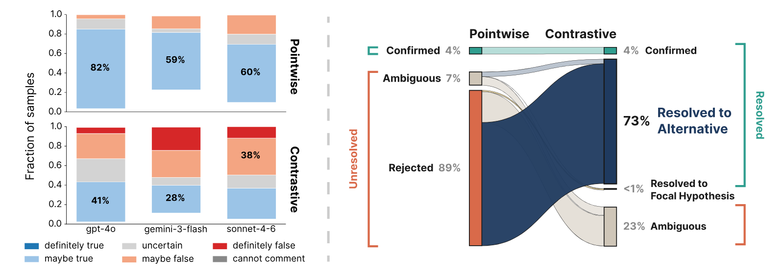
We first ask what high-scoring pointwise surprisal candidates actually represent. Figure 2 (left) shows that pointwise hypothesis proposals concentrate heavily in the “maybe true” prior bin across three belief elicitors (at least 59% for each). This concentration is strongest when the same model, gpt-4o, both proposes and elicits (82%), but remains pronounced under cross-model elicitation. In contrast, explanations drawn from contrast sets produce a much broader prior distribution, with the largest bin containing only 41% of mass (gpt-4o). This suggests that pointwise proposals cluster around hypotheses already considered plausible but uncertain, while contrast sets cover a wider range of competing explanations for the same scientific question.
We call this concentration prior collapse, and it affects which candidates pointwise surprisal ranks highest. Because most pointwise hypotheses begin near the “maybe true” bin, there is limited headroom for confirmatory shifts and much more for disconfirming ones (see Appendix for the scoring rule and its normalization). Consistent with this asymmetry, high-surprisal pointwise candidates in our runs are disproportionately negative. Among the top-50 candidates from each run’s 200 experimental validations, only 4% are confirmed, 7% are ambiguous, and 89% are rejected. Pointwise surprisal thus primarily surfaces evidence against a focal claim, and because the complement is unstructured, that evidence does not identify which alternative explanation is better supported.
To test whether those rejected hypotheses contain recoverable information, we construct a post-hoc contrastive companion for each pointwise hypothesis: we keep the original hypothesis as one explanation, generate alternatives using the same contrast-set proposer, and reuse the same evidence (prompt in Appendix P.3). This uses contrast sets as an evaluation lens: no new experiments are run. The companion generator sees the hypothesis, the dataset’s variables, and the same prior context as a live proposer, but not the analysis, its output, or the verdict, and it is applied whether the hypothesis was confirmed or rejected. On the same evidence, the companion resolves 73% of the 50 candidates to an alternative (Figure 2, right). Counting only confirmations as resolutions, pointwise discovery leaves 96% of them unresolved, against 23% for Contrastive. Because both readings use the same evidence, the difference comes from how the hypothesis space is represented: the same evidence pointwise discovery spends to reject a claim can instead identify what is more plausible.
Having shown that pointwise rejection often contains information that resolves an alternative, we next test whether using contrast sets to guide search directly captures this latent information to resolve more scientific questions. For both methods, we rank candidates by their respective discovery scores (i.e., or surprisal) and evaluate the top- questions retained for inspection. Pointwise baselines cluster together (Figure 3): ranking candidates by surprisal, novelty, or feasibility yields similar numbers of resolved questions. This suggests that the limitation is in the pointwise representation rather than its scoring function since an isolated hypothesis can only be confirmed or rejected. In contrast, Contrastive Discovery produces substantially more resolved questions across budgets: at , it resolves 161.9 questions on average versus 97.2 for pointwise surprisal (+67%).
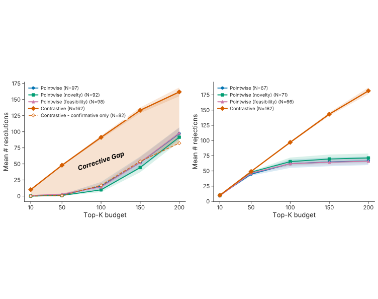
The confirmative-only Contrastive curve shows that the gain is not driven by simply confirming more prior-leading explanations: when restricted to confirmative resolutions, Contrastive Discovery sits at or below the pointwise surprisal baseline (82.2 vs. 97.2 at ), plausibly because , as the search reward, values confirming an already-leading explanation less, so the search pursues such questions less often. The additional yield comes almost entirely from corrective resolutions, where evidence shifts support from the prior-leading explanation to another member of the contrast set. This corrective gap is the information lost in pointwise discovery. There, the same evidence can reject the focal hypothesis, but because the alternative space is collapsed into an unstructured complement, it cannot identify which competing explanation becomes better supported.
Resolving more questions does not come at the expense of ruling out alternatives: placing belief on one explanation leaves at most for the rest, so at the typical size of three, a resolved set almost always rules out at least one alternative (see Appendix Q.2). To count a verdict in either direction for both methods, we report the decisive-unit rate: the fraction of top- units reaching any verdict (confirmed or rejected for pointwise, resolved or ruled out for Contrastive). At , it is for Contrastive versus for pointwise and is higher across all six datasets (Appendix Q.3).
To evaluate which change produces the gain, we isolate three factors in the discovery pipeline: ranking (pointwise surprisal vs. Contrastive ), evaluation (focal hypothesis only vs. full contrast set), and discovery-time construction (contrast set built post-hoc vs. during the discovery run). We compare five variants: pointwise only, +Contrastive ranking, +Contrastive evaluation, +Contrastive ranking & evaluation, and Full Contrastive. Post-hoc variants reuse evidence collected for a pointwise hypothesis with a companion contrast set; Full Contrastive constructs the contrast set during discovery time. We evaluate on three metrics: resolution rate measures whether the update answers the question, realized information gain (IG; the contrastive belief shift , with under pointwise evaluation) measures the magnitude of belief shift, and margin gain measures how much the belief gap between the leading explanation and runner-up changes after observing the evidence (Figure 4).
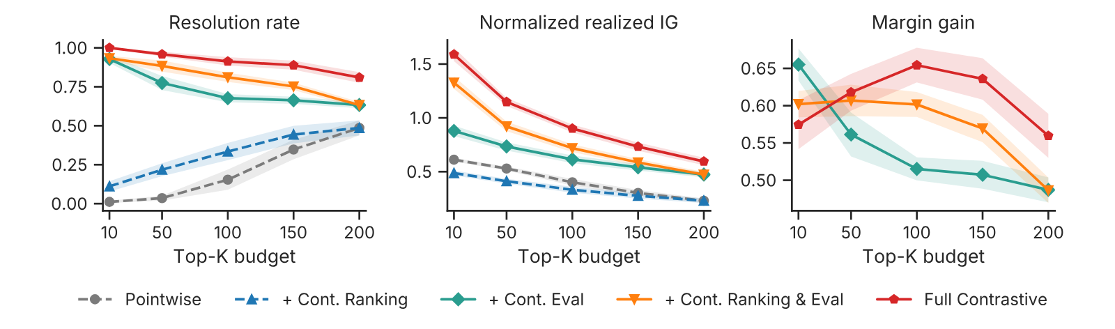
The largest separation comes from changing how evidence is evaluated. Variants with pointwise evaluation remain low in resolution rate (at most 0.22 at ), whereas variants with Contrastive evaluation improve substantially (ranging from 0.77 to 0.96 at ). Once alternatives are explicitly represented, the same evidence can then adjudicate among explanations. Contrastive ranking raises resolution under either evaluator, but under pointwise evaluation it yields lower information gain than pointwise ranking (Figure 4, middle), revealing a ranker–evaluator mismatch: the ranker prioritizes evidence informative over alternatives, while the evaluator collapses that evidence back onto a single focal claim. When Contrastive ranking is paired with Contrastive evaluation, both resolution and realized information gain increase.
Finally, post-hoc companion sets improve over pointwise evaluation, but Full Contrastive leads on all three metrics at almost every top- budget, consistent with alternatives built during discovery shaping the question, analysis plan, and evidence collected. Resolved-question yield is driven primarily by contrastive evaluation, strengthened by contrastive ranking, and highest when alternatives are built during discovery.
Compatibility with pointwise surprisal. The contrastive belief shift stays compatible with the pointwise surprisal signal used by prior work [2]. To compare the two scores on shared candidates, we take the highest-prior hypothesis of each contrast set and score it with pointwise surprisal. The two scores are aligned (Spearman ); where they disagree, candidates ranked higher by Contrastive are often corrective and those ranked higher by pointwise confirmative. Under this single-hypothesis scoring, Contrastive Discovery also matches the pointwise surprisal, novelty, and feasibility baselines in its yield of surprising hypotheses, those whose pointwise surprisal reaches 0.5 (see ).
A resolution only records where one model’s belief settled, so we further validate it against independent references that do not depend on that model.
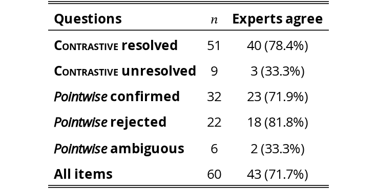
Blinded human expert evaluation. Thirty-eight evaluators with MS or PhD degrees judged 60 questions across all datasets using only the question, candidate explanations, and evidence; a median of 8 rated each item, and we use the majority vote. As Table 1 shows, experts agreed with Contrastive Discovery’s explanation on 78.4% of resolved questions. Of the 17 disagreements across all 60 items, they favored a competing explanation in only three cases; the rest were inconclusive or split. For the pointwise comparison, we used the same 60 questions, evidence, and expert judgments, evaluating only the explanation with the highest prior belief in the contrast set. When pointwise confirmed its hypothesis, experts endorsed 23 of the 32 findings (71.9%) for each method; when pointwise rejected and stopped, they selected the alternative identified by Contrastive Discovery on 81.8%. Evaluators also judged contrast sets well formed on 80% of ratings, flagged a plausible alternative as missing on 15%, and rated the result a substantive finding on 51%. As quality controls, evaluators reliably flagged planted defective sets, and pairing questions with unrelated evidence reduced appropriate-analysis ratings from 73% to 7% (Appendix I).
| Questions | Experts agree | |
|---|---|---|
| Contrastive resolved | 51 | 40 (78.4%) |
| Contrastive unresolved | 9 | 3 (33.3%) |
| Pointwise confirmed | 32 | 23 (71.9%) |
| Pointwise rejected | 22 | 18 (81.8%) |
| Pointwise ambiguous | 6 | 2 (33.3%) |
| All items | 60 | 43 (71.7%) |
View original table
Resolutions follow the evidence. To verify that resolutions follow the evidence rather than the wording of the alternatives, we gave the belief elicitor only the numerical results for 14 claims adapted from DiscoveryBench [32] with documented findings, with no analyst text, the alternatives worded identically across conditions, and their order randomized. Given the coefficient and confidence interval, it ranked the documented answer first in all 11 cases where an interval could be recovered. Holding alternative wording fixed, reversing the evidence’s sign reversed resolutions on all 14 claims, while removing evidence prevented resolution. Separately, recomputing 331 analyses directly from raw data reproduced the agent’s reported statistics on 96.1% (Appendix J).
Agreement across model families. When we re-elicited beliefs on 180 contrast sets with gpt-4o, gemini-3-flash, and claude-sonnet-4-6, all three models chose the same leading explanation on 55% of sets before seeing the evidence and on 88.9% after, and agreement rose in every dataset (see Appendix A).
Incomplete contrast sets. A contrast set that omits the explanation the evidence supports can produce a confident wrong resolution. For 163 questions whose supported explanation was independently identified from recomputed statistics and which the system had originally resolved correctly, we removed that explanation from its contrast set and re-elicited beliefs. The system declined to resolve on 46.6% and resolved to a wrong explanation on 53.4%, mostly to “no detectable effect.” Adding the abstention alternative (§3.4) reduced false resolutions to 0.6%, typically flagging the omission rather than withholding an answer. On re-elicitation of the same intact sets, abstention was never selected, and 162/163 resolved to the supported explanation versus 159/163 without abstention. Our main results use the generated alternatives without abstention: a strict majority of experts identified a missing alternative in only 6 of 60 rated sets (Appendix K).
To test the robustness of the gain in §5.2, we vary key evaluation choices (details in Appendix L).
Joint versus independent scoring. Contrastive Discovery both writes out the alternatives and scores them together in one belief distribution; the gain could come from either. Keeping the contrast sets but scoring each alternative separately with the pointwise elicitor and its threshold resolves 157.8 questions against 161.9 for joint scoring, and both select the same leading alternative on 89.3% of sets. Joint scoring therefore accounts for little of the gain, and contrast sets can be layered onto an agent that keeps its existing pointwise scorer.
Budget. Both methods are given the same number of experimental validations, at similar cost per candidate (61.1k tokens for pointwise against 52.8k for Contrastive). We also recompute the comparison with both methods capped at the same total tokens or the same dollar cost. Contrastive Discovery still resolves more under each: 148.3 against 87.7 at equal tokens and 145.8 against 92.2 at equal dollars.
Thresholds. If our resolution threshold were easier to clear than the pointwise confirmation threshold, we would resolve more questions for that reason alone. Because bounds a share of a distribution over alternatives and bounds a scalar belief, we match the two by how often they accept the same evidence. On 1,543 cases where the pointwise elicitor scored the same evidence for the prior-leading explanation and it stayed the leader, we pair each from 0.60 to 0.90 with the that accepts the closest fraction of cases. Contrastive Discovery resolves more at every matched pair and in each of the six datasets. At our , the matched is 0.695, stricter than the 0.625 we use, so the reported gain is conservative (Appendix E).
Implicit contrast sets. Pointwise discovery might independently propose the alternatives in our contrast sets, allowing post-hoc recovery. Using a separate LLM judge, we compare every pointwise hypothesis against a stratified sample of 300 contrast sets. Among the questions that at least one pointwise hypothesis also addresses, the pointwise hypotheses contain the complete alternative set for only 2.6% within a single run at matched budget, and for only 15.4% after pooling all pointwise runs on the dataset (– that budget). At matched budget, the posterior-leading explanation appears among the pointwise hypotheses 52.0% of the time when the evidence confirms the prior-leading explanation, but only 25.4% when it corrects it. So where pointwise evaluation would reject its hypothesis, it has usually not proposed the explanation the evidence favors (Appendix L).
Recent surveys trace the shift from task-specific automation toward autonomous LLM-driven discovery systems [46, 3]. Related work develops hypothesis-generation and refinement methods [8, 22], alongside pairwise LLM evaluation [28] and scientific argument alignment [9]. In contrast to such settings that generate or evaluate hypotheses individually or in pairs, Contrastive Discovery focuses on how evidence distinguishes a set of mutually exclusive and collectively exhaustive competing explanations for the same question.
This reframing builds on a longer tradition of information-theoretic experimental design, which values experiments by their expected effect on belief [25, 30, 6]. Our objective measures realized posterior–prior belief change through Bayesian surprise [5], following prior evidence-informed LLM discovery work [1, 2]. ClaimSpect [21] also moves beyond binary claim assessment, but organizes existing evidence into non-exclusive aspects rather than constructing mutually exclusive alternatives to be resolved by new analyses. A related line of work also generates research hypotheses from scientific literature, from early text-mining systems [38] to LLM agents [4, 42, 37]. Contrastive Discovery is compatible with this setting because contrastive resolution requires only a scientific question and plausible alternatives. In this work, we focus on open-ended, data-driven discovery [31, 27] over tabular datasets [32, 12], where experiments can be run directly against rich scientific data.
We introduced Contrastive Discovery, which replaces the single hypothesis that a scientific discovery agent proposes and scores with a contrast set of competing explanations. Because only this unit of discovery changes, an existing agent can use contrast sets without changing its architecture, either to re-evaluate evidence it has already collected or to guide its search. Across six domains, contrast sets turn pointwise rejections into resolved questions, almost entirely through corrective resolutions. Ablations trace this gain primarily to evaluating evidence against the full contrast set. In a blinded study, human experts broadly agree with the explanations the system selects on resolved questions. Together, these results support explicit competing explanations as a way for discovery agents to resolve more scientific questions from the same evidence and validation budget.
Our experiments use tabular, observational datasets and a single base agent with a gpt-4o backbone. On such data, a resolution is a statistical rather than a causal finding. Because contrast sets need only an agent’s hypotheses and evidence, we expect the gains to carry over to other discovery agents, which we leave to future work. Contrast sets may also be malformed or omit plausible explanations. Structural audits and expert ratings find most sets well formed (Appendix C and §5.4), and adding an abstention alternative flags omitted explanations (§5.4). Finally, resolution is measured with LLM-elicited beliefs, so resolved-question counts depend on the elicitor, even though most resolutions agree with recomputed statistics and experts (§5.4). Future work should test whether these gains extend to laboratory experiments and longer-horizon interventions.
This material is based on work supported by the AI Research Institutes program supported by the NSF and Intel Corporation under NSF award DMR-2433348. This research is supported in part by the National Science Foundation (IIS-2505098). Research supported by the NVIDIA Academic Grant Program using 4 × RTX PRO 6000 Blackwell GPUs.
References
- [1] D. Agarwal, R. Adamson, A. McCallum, P. Clark, A. Sabharwal, and B. P. Majumder (2026) Evidence-informed llm beliefs for continual scientific discovery. External Links: 2606.29182, Link Cited by: §6.Source
- [2] D. Agarwal, B. P. Majumder, R. Adamson, M. Chakravorty, S. R. Gavireddy, A. Parashar, H. Surana, B. D. Mishra, A. McCallum, A. Sabharwal, and P. Clark (2025) AutoDiscovery: open-ended scientific discovery via bayesian surprise. In The Thirty-ninth Annual Conference on Neural Information Processing Systems, External Links: Link Cited by: Appendix F, §1, §1, §2, §2, §3.5, §3, §4, §4, §5.3, §6.Source
- [3] A. K. Alkan, S. Sourav, M. Jablonska, S. Astarita, R. Chakrabarty, N. Garuda, P. Khetarpal, M. Pióro, D. Tanoglidis, K. G. Iyer, M. S. Polimera, M. J. Smith, T. Ghosal, M. Huertas-Company, S. Kruk, K. Schawinski, and I. Ciucă (2025) A survey on hypothesis generation for scientific discovery in the era of large language models. External Links: 2504.05496, Link Cited by: §6.Source
- [4] J. Baek, S. K. Jauhar, S. Cucerzan, and S. J. Hwang (2025) ResearchAgent: iterative research idea generation over scientific literature with large language models. In Proceedings of the 2025 Conference of the Nations of the Americas Chapter of the Association for Computational Linguistics: Human Language Technologies (Volume 1: Long Papers), L. Chiruzzo, A. Ritter, and L. Wang (Eds.), Albuquerque, New Mexico, pp. 6709–6738. External Links: Link, Document, ISBN 979-8-89176-189-6 Cited by: §1, §2, §4, §6.SourceSource
- [5] P. Baldi and L. Itti (2010) Of bits and wows: a bayesian theory of surprise with applications to attention. Neural Netw. 23 (5), pp. 649–666. External Links: ISSN 0893-6080, Link, Document Cited by: §6.SourceSource
- [6] K. Chaloner and I. Verdinelli (1995) Bayesian Experimental Design: A Review. Statistical Science 10 (3), pp. 273 – 304. External Links: Document, Link Cited by: §6.SourceSource
- [7] R. Coulom (2007) Efficient selectivity and backup operators in monte-carlo tree search. In Computers and Games, H. J. van den Herik, P. Ciancarini, and H. H. L. M. (. Donkers (Eds.), Berlin, Heidelberg, pp. 72–83. External Links: ISBN 978-3-540-75538-8 Cited by: §4.
- [8] S. Duan, Y. Tian, Q. Bing, and X. Shao (2025) Bayes-entropy collaborative driven agents for research hypotheses generation and optimization. External Links: 2508.01746, Link Cited by: §6.Source
- [9] Y. Gao, N. Gu, J. Lam, J. Henderson, and R. Hahnloser (2024) Evaluating unsupervised argument aligners via generation of conclusions of structured scientific abstracts. In Proceedings of the 18th Conference of the European Chapter of the Association for Computational Linguistics (Volume 2: Short Papers), Y. Graham and M. Purver (Eds.), St. Julian’s, Malta, pp. 151–160. External Links: Link, Document Cited by: §6.SourceSource
- [10] A. Garikaparthi, M. Patwardhan, L. Vig, and A. Cohan (2025) IRIS: interactive research ideation system for accelerating scientific discovery. In Proceedings of the 63rd Annual Meeting of the Association for Computational Linguistics (Volume 3: System Demonstrations), P. Mishra, S. Muresan, and T. Yu (Eds.), Vienna, Austria, pp. 592–603. External Links: Link, Document, ISBN 979-8-89176-253-4 Cited by: §1, §2, §4, §4.SourceSource
- [11] J. Gottweis, W. Weng, A. Daryin, T. Tu, A. Palepu, P. Sirkovic, A. Myaskovsky, F. Weissenberger, K. Rong, R. Tanno, K. Saab, D. Popovici, J. Blum, F. Zhang, K. Chou, A. Hassidim, B. Gokturk, A. Vahdat, P. Kohli, Y. Matias, A. Carroll, K. Kulkarni, N. Tomasev, Y. Guan, V. Dhillon, E. D. Vaishnav, B. Lee, T. R. D. Costa, J. R. Penadés, G. Peltz, Y. Xu, A. Pawlosky, A. Karthikesalingam, and V. Natarajan (2025) Towards an ai co-scientist. External Links: 2502.18864, Link Cited by: §1, §1, §2, §4.Source
- [12] K. Gu, R. Shang, R. Jiang, K. Kuang, R. Lin, D. Lyu, Y. Mao, Y. Pan, T. Wu, J. Yu, Y. Zhang, T. M. Zhang, L. Zhu, M. A. Merrill, J. Heer, and T. Althoff (2024) BLADE: benchmarking language model agents for data-driven science. In Findings of the Association for Computational Linguistics: EMNLP 2024, Y. Al-Onaizan, M. Bansal, and Y. Chen (Eds.), Miami, Florida, USA, pp. 13936–13971. External Links: Link, Document Cited by: §4, §6.SourceSource
- [13] J. S. Gupta, S. M. Tawseeq, H. S. I, S. K. Singh, Y. K. Singla, D. Doermann, R. R. Shah, and B. Krishnamurthy (2025) ExperiGen: data driven hypothesis generation with experimental verification. External Links: Link Cited by: §1.Source
- [14] R. Ha, C. Li, R. Pu, L. Zhang, X. Zhang, and S. Su (2025) DSG-MCTS: a dynamic strategy-guided Monte Carlo tree search for diversified reasoning in large language models. In Proceedings of the 2025 Conference on Empirical Methods in Natural Language Processing, C. Christodoulopoulos, T. Chakraborty, C. Rose, and V. Peng (Eds.), Suzhou, China, pp. 10530–10544. External Links: Link, Document, ISBN 979-8-89176-332-6 Cited by: §4.SourceSource
- [15] M. K. Horton, P. Huck, R. X. Yang, J. M. Munro, S. Dwaraknath, A. M. Ganose, R. S. Kingsbury, M. Wen, J. X. Shen, T. S. Mathis, A. D. Kaplan, K. Berket, J. Riebesell, J. George, A. S. Rosen, E. W. C. Spotte-Smith, M. J. McDermott, O. A. Cohen, A. Dunn, M. C. Kuner, G. Rignanese, G. Petretto, D. Waroquiers, S. M. Griffin, J. B. Neaton, D. C. Chrzan, M. Asta, G. Hautier, S. Cholia, G. Ceder, S. P. Ong, A. Jain, and K. A. Persson (2025) Accelerated data-driven materials science with the materials project. Nature Materials 24 (10), pp. 1522–1532. External Links: ISSN 1476-4660, Document, Link Cited by: §4.SourceSource
- [16] X. Hu, H. Fu, J. Wang, Y. Wang, Z. Li, R. Xu, Y. Lu, Y. Jin, L. Pan, and Z. Lan (2025) NOVA: an iterative planning framework for enhancing scientific innovation with large language models. In Findings of the Association for Computational Linguistics: ACL 2025, W. Che, J. Nabende, E. Shutova, and M. T. Pilehvar (Eds.), Vienna, Austria, pp. 21330–21359. External Links: Link, Document, ISBN 979-8-89176-256-5 Cited by: §4.SourceSource
- [17] K. Huang, Y. Jin, R. Li, M. Y. Li, E. Candes, and J. Leskovec (2025) Automated hypothesis validation with agentic sequential falsifications. In Forty-second International Conference on Machine Learning, External Links: Link Cited by: §1, §2.Source
- [18] L. Itti and P. Baldi (2005) Bayesian surprise attracts human attention. In Advances in Neural Information Processing Systems, Y. Weiss, B. Schölkopf, and J. Platt (Eds.), Vol. 18, pp. . External Links: Link Cited by: §1, §3.3, §3.Source
- [19] P. Jansen, O. Tafjord, M. Radensky, P. Siangliulue, T. Hope, B. D. Mishra, B. P. Majumder, D. S. Weld, and P. Clark (2025) CodeScientist: end-to-end semi-automated scientific discovery with code-based experimentation. External Links: 2503.22708, Link Cited by: §1.Source
- [20] Z. Jiang, D. Schmidt, D. Srikanth, D. Xu, I. Kaplan, D. Jacenko, and Y. Wu (2025) AIDE: ai-driven exploration in the space of code. External Links: 2502.13138, Link Cited by: §4.Source
- [21] P. Kargupta, R. Tian, and J. Han (2025) Beyond true or false: retrieval-augmented hierarchical analysis of nuanced claims. In Proceedings of the 63rd Annual Meeting of the Association for Computational Linguistics (Volume 1: Long Papers), W. Che, J. Nabende, E. Shutova, and M. T. Pilehvar (Eds.), Vienna, Austria, pp. 29664–29679. External Links: Link, Document, ISBN 979-8-89176-251-0 Cited by: §6.SourceSource
- [22] Y. Ke, K. George, K. Pandya, D. Blumenthal, M. Sprang, G. Großmann, S. Vollmer, and D. A. Selby (2025) BioDisco: multi-agent hypothesis generation with dual-mode evidence, iterative feedback and temporal evaluation. External Links: 2508.01285, Link Cited by: §6.Source
- [23] L. Kocsis and C. Szepesvári (2006) Bandit based monte-carlo planning. In Proceedings of the 17th European Conference on Machine Learning, ECML’06, Berlin, Heidelberg, pp. 282–293. External Links: ISBN 354045375X, Link, Document Cited by: §4.SourceSource
- [24] R. Li, L. Jing, and X. Du (2024) Learning to generate research idea with dynamic control. External Links: Link Cited by: §1, §2, §4.Source
- [25] D. V. Lindley (1956) On a Measure of the Information Provided by an Experiment. The Annals of Mathematical Statistics 27 (4), pp. 986 – 1005. External Links: Document, Link Cited by: §6.SourceSource
- [26] P. Lipton (2004) Inference to the best explanation. 2nd edition, Routledge. External Links: ISBN 9780415242035 Cited by: §1.
- [27] H. Liu, S. Huang, J. Hu, Y. Zhou, and C. Tan (2026) HypoBench: towards systematic and principled benchmarking for hypothesis generation. External Links: 2504.11524, Link Cited by: §6.Source
- [28] A. Liusie, P. Manakul, and M. J. F. Gales (2024) LLM comparative assessment: zero-shot nlg evaluation through pairwise comparisons using large language models. External Links: 2307.07889, Link Cited by: §6.Source
- [29] C. Lu, C. Lu, R. T. Lange, J. Foerster, J. Clune, and D. Ha (2024) The ai scientist: towards fully automated open-ended scientific discovery. External Links: 2408.06292, Link Cited by: §1.Source
- [30] D. J. C. MacKay (1992) Information-based objective functions for active data selection. Neural Computation 4 (4), pp. 590–604. External Links: ISSN 0899-7667, Document Cited by: §6.Source
- [31] B. P. Majumder, H. Surana, D. Agarwal, S. Hazra, A. Sabharwal, and P. Clark (2024) Data-driven discovery with large generative models. External Links: 2402.13610, Link Cited by: §1, §6.Source
- [32] B. P. Majumder, H. Surana, D. Agarwal, B. D. Mishra, A. Meena, A. Prakhar, T. Vora, T. Khot, A. Sabharwal, and P. Clark (2025) DiscoveryBench: towards data-driven discovery with large language models. In The Thirteenth International Conference on Learning Representations, External Links: Link Cited by: Appendix N, §4, §5.4, §6.Source
- [33] A. Novikov, N. Vũ, M. Eisenberger, E. Dupont, P. Huang, A. Z. Wagner, S. Shirobokov, B. Kozlovskii, F. J. R. Ruiz, A. Mehrabian, M. P. Kumar, A. See, S. Chaudhuri, G. Holland, A. Davies, S. Nowozin, P. Kohli, and M. Balog (2025) AlphaEvolve: a coding agent for scientific and algorithmic discovery. External Links: 2506.13131, Link Cited by: §1.Source
- [34] B. Qi, K. Zhang, K. Tian, H. Li, Z. Chen, S. Zeng, E. Hua, H. Jinfang, and B. Zhou (2024) Large language models as biomedical hypothesis generators: a comprehensive evaluation. In First Conference on Language Modeling, External Links: Link Cited by: §1, §4.Source
- [35] S. Schmidgall, Y. Su, Z. Wang, X. Sun, J. Wu, X. Yu, J. Liu, M. Moor, Z. Liu, and E. Barsoum (2025) Agent laboratory: using llm agents as research assistants. External Links: 2501.04227, Link Cited by: §1.Source
- [36] SDSS Collaboration, G. A. Pallathadka, M. Aghakhanloo, J. Aird, A. Almeida, S. Amrita, F. Anders, S. F. Anderson, S. Arseneau, C. G. Avila, S. Aviram, C. Aydar, C. Badenes, J. K. Barrera-Ballesteros, F. E. Bauer, A. Behmard, M. Berg, F. Besser, C. M. Bidin, D. Bizyaev, G. Blanc, M. R. Blanton, J. Bovy, W. N. Brandt, J. R. Brownstein, J. Buchner, E. Bulbul, J. N. Burchett, L. Carigi, J. K. Carlberg, A. R. Casey, P. Chakraborty, J. Chanamé, V. Chandra, C. Chiappini, I. Chilingarian, J. Comparat, K. Covey, N. Crumpler, K. Cunha, E. D’Onghia, X. Dai, J. Darling, M. Davis, N. D. Lee, N. Deacon, J. E. M. Delgado, S. Demasi, M. Demianenko, D. Demke, J. Donor, N. Drory, M. A. V. Durango, T. Dwelly, O. Egorov, E. Egorova, K. El-Badry, M. Eracleous, X. Fan, E. Farr, D. P. Finkbeiner, L. Fries, P. Frinchaboy, N. P. G. Fusillo, L. D. S. Félix, B. Gaensicke, E. Galligan, P. García, J. Gelfand, K. Grabowski, E. Grebel, P. J. Green, H. Greve, C. Grier, E. Griffith, P. Guetzoyan, P. Gupta, Z. Hackshaw, P. B. Hall, K. Hawkins, V. Hegedűs, S. Hekker, T. M. Herbst, J. J. Hermes, L. Hernández-García, P. Hiremath, D. W. Hogg, J. Holtzman, K. Horne, D. Horta, Y. Huang, B. Hutchinson, M. Häberle, H. J. Ibarra-Medel, A. P. Ji, P. Jofre, J. W. Johnson, J. Johnson, E. J. Johnston, M. Kaldor, I. Katkov, A. Khalatyan, S. Khoperskov, R. Klessen, M. Kluge, A. M. Koekemoer, J. A. Kollmeier, M. Kounkel, K. Kreckel, D. Krishnarao, M. Krumpe, I. Lacerna, C. Laporte, S. Lepine, J. Li, F. Liang, G. Limberg, X. Liu, S. Loebman, K. Long, Y. Lu, M. Lucey, A. Z. Lugo-Aranda, M. L. M. Martinez-Aldama, K. McKinnon, I. Medan, A. Merloni, S. Morrison, N. Myers, S. Mészáros, J. Müller-Horn, S. Nepal, M. Ness, D. Nidever, C. Nitschelm, A. Oravetz, J. Otto, K. Pan, F. P. Paolino, C. A. N. Peñaloza, M. Pinsonneault, M. T. Popp, A. Price-Whelan, N. Pulatova, A. B. Queiroz, J. Raddick, A. Rankine, H. Rix, C. Román-Zúñiga, D. F. Rosso, J. Runnoe, S. M. Saad, M. Salvato, S. F. Sanchez, N. Sattler, A. Saydjari, C. Sayres, K. Schlaufman, D. P. Schneider, A. Schwope, L. M. Seaton, R. Seeburger, J. Serna, S. Sharma, Y. Shen, A. Sinha, B. Sizemore, M. Sniegowska, Y. Song, D. Souto, K. Stassun, M. Steinmetz, Z. Stone, A. Stone-Martinez, G. S. Stringfellow, A. M. Sánchez, J. Sánchez-Gallego, J. Tan, J. Tayar, R. Thai, A. Thakar, P. Thibodeaux, Y. Ting, A. Tkachenko, B. Trakhtenbrot, J. G. F. Trincado, N. Troup, J. R. Trump, N. Ulloa, R. P. V. der Marel, P. Vera, S. Villanova, J. Villaseñor, J. Wang, Z. Way, A. Weijmans, A. Wheeler, J. C. Wilson, A. Wofford, T. Wong, Q. Wu, D. Wylezalek, X. Xue, R. Yan, Q. Yang, N. Zakamska, E. Zari, G. Zasowski, G. Zeltyn, Z. Zheng, C. Zucker, and R. de J. Zermeño (2025) The nineteenth data release of the sloan digital sky survey. External Links: 2507.07093, Link Cited by: §4.Source
- [37] C. Si, D. Yang, and T. Hashimoto (2024) Can llms generate novel research ideas? a large-scale human study with 100+ nlp researchers. External Links: 2409.04109, Link Cited by: §6.Source
- [38] S. Spangler, A. D. Wilkins, B. J. Bachman, M. Nagarajan, T. Dayaram, P. Haas, S. Regenbogen, C. R. Pickering, A. Comer, J. N. Myers, I. Stanoi, L. Kato, A. Lelescu, J. J. Labrie, N. Parikh, A. M. Lisewski, L. Donehower, Y. Chen, and O. Lichtarge (2014) Automated hypothesis generation based on mining scientific literature. In Proceedings of the 20th ACM SIGKDD International Conference on Knowledge Discovery and Data Mining, KDD ’14, New York, NY, USA, pp. 1877–1886. External Links: ISBN 9781450329569, Link, Document Cited by: §6.SourceSource
- [39] H. W. Sprueill, C. Edwards, K. Agarwal, M. V. Olarte, U. Sanyal, C. Johnston, H. Liu, H. Ji, and S. Choudhury (2024) ChemReasoner: heuristic search over a large language model’s knowledge space using quantum-chemical feedback. External Links: 2402.10980, Link Cited by: §4.Source
- [40] E. Toledo, K. Hambardzumyan, M. Josifoski, R. Hazra, N. Baldwin, A. Audran-Reiss, M. Kuchnik, D. Magka, M. Jiang, A. M. Lupidi, A. Lupu, R. Raileanu, K. Niu, T. Shavrina, J. Gagnon-Audet, M. Shvartsman, S. Sodhani, A. H. Miller, A. Charnalia, D. Dunfield, C. Wu, P. Stenetorp, N. Cancedda, J. N. Foerster, and Y. Bachrach (2025) AI research agents for machine learning: search, exploration, and generalization in mle-bench. External Links: 2507.02554, Link Cited by: §4.Source
- [41] B. C. van Fraassen (1980) The scientific image. Oxford University Press. External Links: ISBN 9780191597473 Cited by: §1.
- [42] Q. Wang, D. Downey, H. Ji, and T. Hope (2024) SciMON: scientific inspiration machines optimized for novelty. In Proceedings of the 62nd Annual Meeting of the Association for Computational Linguistics (Volume 1: Long Papers), pp. 279–299. External Links: Link, Document Cited by: §6.SourceSource
- [43] Y. Yamada, R. T. Lange, C. Lu, S. Hu, C. Lu, J. Foerster, J. Clune, and D. Ha (2025) The ai scientist-v2: workshop-level automated scientific discovery via agentic tree search. External Links: 2504.08066, Link Cited by: §1, §4.Source
- [44] Z. Yang, W. Liu, B. Gao, Y. Liu, W. Li, T. Xie, L. Bing, W. Ouyang, E. Cambria, and D. Zhou (2025) MOOSE-chem2: exploring llm limits in fine-grained scientific hypothesis discovery via hierarchical search. External Links: 2505.19209, Link Cited by: §4.Source
- [45] M. Yuksekgonul, D. Koceja, X. Li, F. Bianchi, J. McCaleb, X. Wang, J. Kautz, Y. Choi, J. Zou, C. Guestrin, and Y. Sun (2026) Learning to discover at test time. External Links: 2601.16175, Link Cited by: §1.Source
- [46] T. Zheng, Z. Deng, H. T. Tsang, W. Wang, J. Bai, Z. Wang, and Y. Song (2025) From automation to autonomy: a survey on large language models in scientific discovery. In Proceedings of the 2025 Conference on Empirical Methods in Natural Language Processing, C. Christodoulopoulos, T. Chakraborty, C. Rose, and V. Peng (Eds.), Suzhou, China, pp. 17733–17750. External Links: Link, Document, ISBN 979-8-89176-332-6 Cited by: §6.SourceSource
A useful and effective hypothesis generator should produce claims that span the prior-belief axis, because scientific discovery is bidirectional: evidence may either support an initially unlikely claim or refute an initially plausible one. We audit LLM-elicited priors for hypotheses generated by free-form prompting (pointwise) and contrastive partitioning (Contrastive), and identify prior collapse, a failure of free-form generation that the contrastive construction structurally mitigates.
We fix the hypothesis generator to gpt-4o and re-elicit beliefs using three independent elicitors: gpt-4o, gemini-3-flash, and claude-sonnet-4-6. For each of six datasets, we sample 90 pointwise hypotheses and 30 Contrastive sets, stratified by tree level. A pointwise node contains a single hypothesis, whereas a Contrastive node contains a partition of mutually exclusive cells (typically ), each treated as a standalone hypothesis for the per-cell label analysis. This gives us a sample of 540 pointwise hypotheses and 180 Contrastive sets (573 Contrastive cells).
Following our generation process exactly, for each hypothesis (or contrast cell) and elicitor, we draw 10 categorical belief samples over five labels: definitely_true, maybe_true, uncertain, maybe_false, and definitely_false. We map these labels to scores , , , , and , respectively, and aggregate them into a posterior under a Jeffreys prior. We use the Beta mean as the per-hypothesis belief score. To measure cross-elicitor agreement on Contrastive at the unit of analysis the runtime metric actually uses, we additionally elicit set-level partition allocations: each elicitor distributes 100 probability points jointly over the cells of a set (5 samples for each set, elicitor, and prior or posterior call, averaged into one -vector).
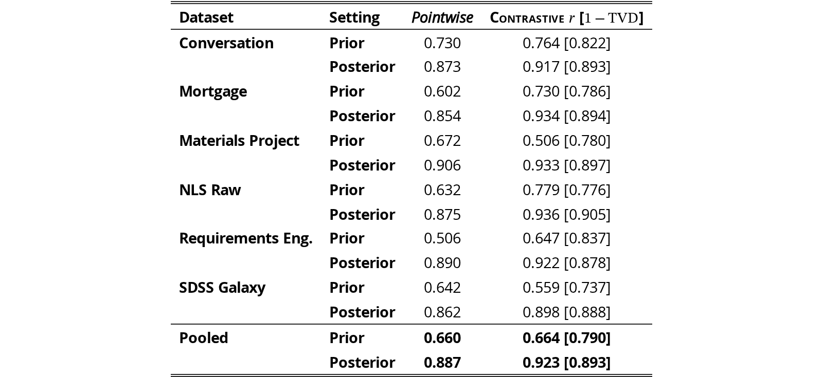
The prior collapse on pointwise priors does not imply that elicitors are simply noisy. Table 2 shows cross-elicitor agreement on per-hypothesis ranks (pointwise, Spearman ) and on per-set partition allocations (Contrastive, mean per-set Pearson , with as a total-variation similarity robustness check at the partition level the runtime metric actually uses). On both methods, evidence sharply raises agreement: pooled rises on pointwise, pooled rises on Contrastive (paired Wilcoxon for both, all per-dataset cells significant under both Bonferroni and Benjamini–Hochberg corrections over 24 tests). The symmetry of this convergence argues against elicitor noise as the source of the unreliability we observe at the prior step: when given evidence, the elicitors are more cross-elicitor consistent on both methods. What is not symmetric is the prior collapse, which is a property of the free-form generator that the elicitor cannot fix. Constructing hypotheses as a mutually exclusive partition rather than independent free-form claims reduces the collapse at the source. This matters because discovery is bidirectional: maximal information gain either comes from evidence refuting an initially plausible claim or from evidence supporting an initially unlikely one, and each requires the generator to propose hypotheses on the corresponding side of the prior axis. Under pointwise prior collapse, the refutational direction dominates. Because the generator rarely produces claims with low elicited prior, discoveries in which evidence confirms an initially unlikely claim are rare. Contrastive’s partition tends to include lower-prior cells by forcing explicit alternatives, restoring access to the full prior axis on which discovery operates, while leaving the elicitor’s evidence-driven posterior convergence intact.
Agreement on ranks and allocations does not show that the families agree on which explanation the evidence supports, so we also compared their leading cells. On the same 180 contrast sets, all three families lead with the same explanation on 55.0% of sets before the evidence (99 of 180; chance, given each family’s observed choice frequencies, is 21.8%) and on 88.9% after it (160 of 180; McNemar exact ). The rise holds in every dataset (Conversation 6390%, Mortgage 6390%, Materials 3793%, NLS 7387%, Requirements 4790%, SDSS 4783%). How often each family crosses differs (gpt-4o 77.2%, gemini-3-flash 86.1%, claude-sonnet-4-6 67.8%), so the resolution rate depends on the elicitor while the leading explanation does not. Three families that start apart and converge after reading the evidence are hard to explain as one model agreeing with itself. One caveat remains: all three read the same gpt-4o analyst summary, so part of the convergence could come from shared framing rather than the evidence alone.
| Dataset | Setting | Pointwise | Contrastive [] |
|---|---|---|---|
| Conversation | Prior | 0.730 | 0.764 [0.822] |
| Posterior | 0.873 | 0.917 [0.893] | |
| Mortgage | Prior | 0.602 | 0.730 [0.786] |
| Posterior | 0.854 | 0.934 [0.894] | |
| Materials Project | Prior | 0.672 | 0.506 [0.780] |
| Posterior | 0.906 | 0.933 [0.897] | |
| NLS Raw | Prior | 0.632 | 0.779 [0.776] |
| Posterior | 0.875 | 0.936 [0.905] | |
| Requirements Eng. | Prior | 0.506 | 0.647 [0.837] |
| Posterior | 0.890 | 0.922 [0.878] | |
| SDSS Galaxy | Prior | 0.642 | 0.559 [0.737] |
| Posterior | 0.862 | 0.898 [0.888] | |
| Pooled | Prior | 0.660 | 0.664 [0.790] |
| Posterior | 0.887 | 0.923 [0.893] |
View original table
Our contrastive score relies on elicited prior and posterior distributions over each contrast set. To reduce stochastic variation, the production pipeline draws point-allocation samples for each prior and posterior elicitation, normalizes each valid allocation to the simplex, and averages the resulting distributions before computing contrastive belief shift. This appendix evaluates whether is a sufficient cost–stability tradeoff for the quantities used by the pipeline.
We analyze contrast sets with complete prior and posterior elicitations. For contrast set , let denote prior samples and denote posterior samples. The production estimates are
We focus on the two derived quantities used downstream: the realized contrastive information gain
and posterior concentration
We first measure within-contrast-set dispersion using the mean pairwise total variation distance among the five elicited distributions. Prior samples are more dispersed than posterior samples: the pooled mean pairwise TVD is for priors and for posteriors. This gap is expected, since prior elicitation is performed before observing evidence, while posterior elicitation is conditioned on the experiment result. The higher prior dispersion is not itself a failure mode; it reflects uncertainty before evidence is observed. What matters downstream is whether the averaged prior and posterior produce stable belief-shift scores. Figure 5 shows the full CDF, with of posterior contrast sets below pairwise TVD .
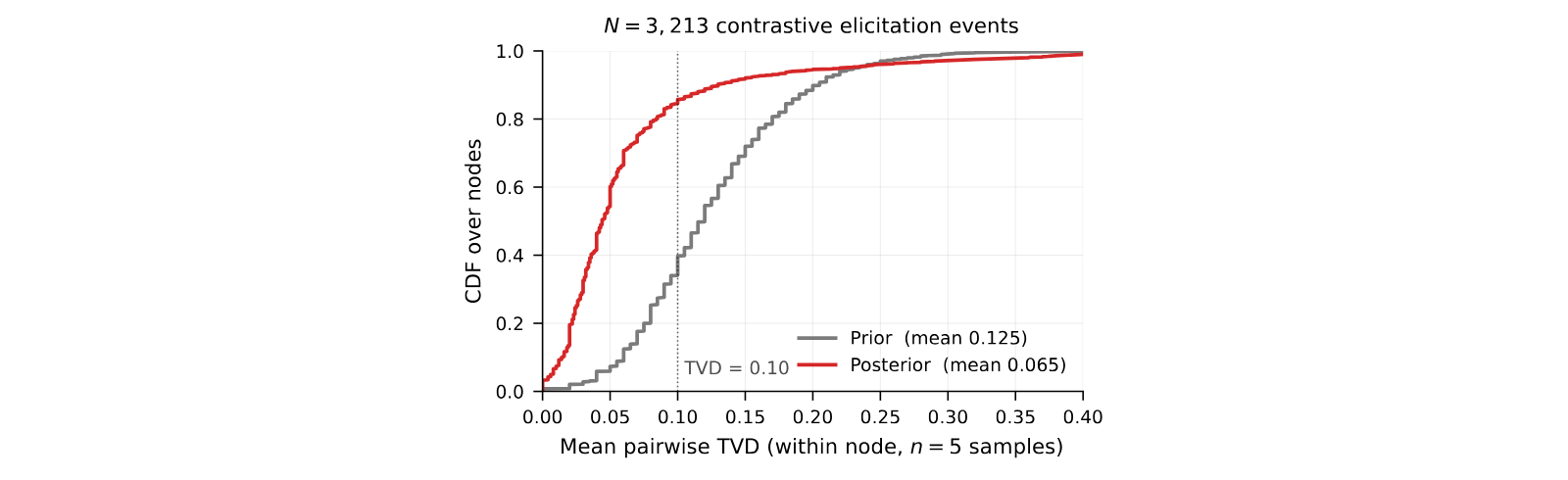
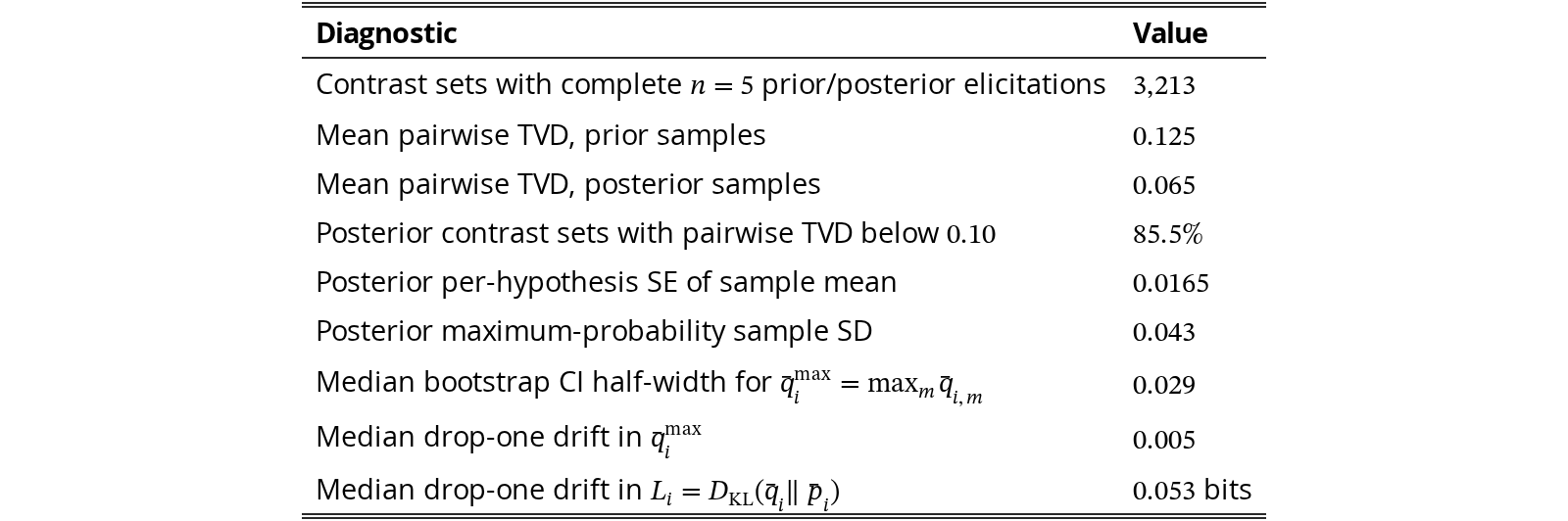
Table 3 reports the diagnostics most relevant to the choice of . The posterior mean has an average per-hypothesis standard error of , corresponding to about points on the -point allocation scale. The posterior concentration is stable under resampling: its median bootstrap CI half-width is , and dropping any one of the five samples changes it by only in median. The KL score depends on both the prior and posterior estimates, and is therefore the relevant joint stability check for the discovery score. Although is noisier than , as expected for a nonlinear function of two finite-sample distributions, its median drop-one drift is only bits. These sensitivities indicate that the production score is not typically driven by a single elicitation sample.
Increasing would further reduce the standard error, but only at the usual rate while increasing elicitation cost linearly. We therefore use as a practical tradeoff: it reduces elicitation variance enough for ranking and aggregate analysis while keeping belief elicitation cost manageable.
| Diagnostic | Value |
|---|---|
| Contrast sets with complete prior/posterior elicitations | |
| Mean pairwise TVD, prior samples | |
| Mean pairwise TVD, posterior samples | |
| Posterior contrast sets with pairwise TVD below | |
| Posterior per-hypothesis SE of sample mean | |
| Posterior maximum-probability sample SD | |
| Median bootstrap CI half-width for | |
| Median drop-one drift in | |
| Median drop-one drift in | bits |
View original table
Contrastive Discovery assumes that each contrast set defines a well-formed partition of possible analysis outcomes. In particular, the explanations in a contrast set should be mutually exclusive and collectively exhaustive (MECE): any plausible result of the planned analysis should support at most one explanation, and the set should not omit an obvious residual outcome. The generator prompt (Appendix P) asks for one of a fixed set of partition templates, a residual outcome, and a quantitative criterion that maps the planned analysis to each alternative; this audit checks the sets it actually produced.
We extracted parseable contrast sets from the full Contrastive runs across datasets and runs. From this pool, we drew a frozen stratified sample of contrast sets, stratifying by the requested partitioning dimension and by the number of hypotheses in the set. This intentionally oversamples rare partition types, making failure modes easier to inspect.
Each sampled contrast set was judged by gpt-4o using two independent passes, with randomized-order votes per pass. The first pass identified pairs of hypotheses that were not logically distinct, including paraphrases, redundant hypotheses, and subsumption relationships. The second pass assigned structural failure tags, including missing residual outcome, redundant hypothesis, subsumption, insufficient number of hypotheses, and inherently non-MECE structure. We classify a contrast set as structurally MECE if no overlap pair, missing-residual, redundancy, subsumption, or inherently non-MECE flag receives at least votes. Insufficient granularity is evaluated separately and does not count as a structural failure. We use this supermajority rule because manual inspection showed that unanimity misses recurring redundancy failures, while simple majority admits more judge noise.
Under the primary rule, sampled contrast sets are structurally MECE (Table 4), corresponding to a raw audit pass rate of . Reweighting the stratified sample back to the full -item pool gives an estimated population pass rate of with a stratified bootstrap 95% confidence interval of . The conclusion is stable across reasonable vote thresholds: the raw pass rate is under a rule and under a rule.
| Quantity | Count / estimate | Rate |
|---|---|---|
| Structurally MECE sampled contrast sets | ||
| Design-weighted population estimate | – | |
| 95% stratified bootstrap CI | – | |
| Overlap or redundancy failures | ||
| Inherently non-MECE mechanism failures |
View original table
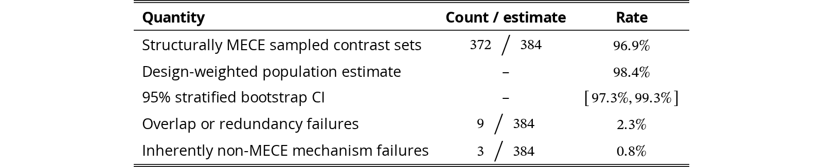
The non-MECE cases are concentrated in two recurring patterns. First, of the failures contain overlapping or redundant hypotheses. These usually occur when the proposer includes two versions of a null or residual outcome. For example, one contrast set contains both “association disappears after controlling for PhD prestige” and “no effect of male contributions on total citations.” These are not exclusive outcomes; both describe the absence of a residual association. Another contrast set contains both “distribution does not follow a specific crystal system” and “no pattern across crystal systems,” which again duplicate the same residual hypothesis.
Second, failures arise from mechanism-style contrast sets that are not naturally MECE. These contrast sets ask the hypotheses to distinguish causal pathways, such as whether residence type affects later wealth through social capital or through initial economic advantage. Without stronger identification assumptions, these mechanisms are not mutually exclusive and may not be empirically separable from the proposed analysis. These cases suggest that mechanism-discriminating templates should either be restricted to observationally distinguishable outcomes or excluded from automatic MECE generation.
The audit above uses a judge from the same provider as the proposer, so we re-ran it on the same 384 sets with Claude Sonnet, keeping the prompts, the two passes, and the rule (Table 5). The cross-provider judge passes 87.0% of sets (91.4% design-weighted) against 96.9% (98.4%) for gpt-4o, flagging 50 sets where gpt-4o flagged 12. The same-provider judge is the more lenient of the two, so we report both figures and carry the stricter one. The disagreement runs almost entirely one way (on the overlap check, 24 sets flagged only by Sonnet against 3 flagged only by gpt-4o), and the extra flags are mostly alternatives that overlap or entail one another. They concentrate by question type: half of the mechanism-discriminating sets and 40% of the ordering sets fail, against none of the directional sets. A structural audit cannot tell whether a plausible explanation is missing altogether; for that, the human raters of Appendix I, who judged the set well formed on 80% of ratings and flagged a missing alternative on 15%, are the external estimate.
| Judge | Provider | Raw pass | Design-weighted pass | Sets flagged |
|---|---|---|---|---|
| gpt-4o (same provider as proposer) | OpenAI | 96.9% | 98.4% | 12 |
| Claude Sonnet | Anthropic | 87.0% | 91.4% | 50 |
View original table

Of the 50 flagged sets, 48 link to a recorded run. On 19 of them the system never reached the resolution threshold, so nothing was reported. Of the 29 resolved questions, 7 selected a member of a judge-named overlapping pair, making those resolutions ambiguous; the other 22 were not identified as implicated by this check. Those 7 are 2.3% of the 302 resolutions in the audited sample, or 1.4% reweighted to the corpus (the audit oversamples risky question types). Two further checks point the same way. Mechanically merging each overlapping pair into one alternative, without re-eliciting beliefs, changes the leading explanation on none of the 379 sets that link to a recorded run, and would newly resolve up to 8 questions left open. Flagged sets also reach the threshold less often than clean ones (60.5% against 85.0% design-weighted, a 24-percentage-point gap with 95% CI 10 to 40), as expected when belief splits between two alternatives that mean the same thing. The defect therefore costs findings rather than inventing them; these are patterns in the logged runs, not a re-elicitation. The residual is small: seven resolutions are ambiguous between two overlapping alternatives, and 19 of the 48 flagged sets could not be tested because the judge named no pair. Whether an explanation is missing altogether is a separate failure, tested in Appendix K.
This audit supports the structural premise of Contrastive: the generated contrast sets usually define valid partitions of the analysis outcome space. The remaining failures are not arbitrary incoherence. They are concentrated in a small number of recognizable template errors, primarily duplicated residual hypotheses and mechanism-style hypotheses that cannot be cleanly partitioned without additional assumptions. We therefore treat MECE structure as satisfied for most sets, while using these failure modes to identify targeted prompt and template improvements. Because a same-provider judge is the more lenient, we carry the cross-provider figure of 87.0% as the conservative estimate.
Contrastive Discovery elicits two probability distributions over the explanations in a contrast set: a prior distribution before observing the analysis result and a posterior distribution after observing it. Since language models can be sensitive to list position, these probabilities could depend on the order in which hypotheses are shown. We therefore randomize the hypothesis order independently for each elicitation call, then invert the permutation before computing priors, posteriors, KL, or any downstream statistic.
We validate this choice with two checks, summarized in Table 6. First, we run a controlled permutation study on four contrast sets from two datasets, with each set evaluated under five different hypothesis orderings. We compare a canonical protocol, which preserves the displayed ordering, against the randomized protocol used in our experiments. After each call, all probabilities are mapped back to the same canonical hypothesis identities. We then measure pairwise consistency across orderings using total variation distance (TVD), where lower TVD means the elicited distribution is less affected by presentation order. Second, we run two parallel Contrastive runs on BLADE Mortgage that differ only in whether hypothesis order is randomized. This checks whether randomization changes the aggregate scale of the elicited KL updates or posterior confidence.
| Pairwise consistency | canonical | randomized | ratio |
|---|---|---|---|
| Prior pairwise TVD | |||
| Posterior pairwise TVD | |||
| Aggregate belief statistics | canonical | randomized | [95% CI] |
View original table
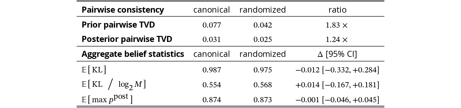
Table 6 shows that randomization improves pairwise consistency across displayed hypothesis orderings. The effect is strongest for the prior distribution: prior pairwise TVD falls from to , a reduction in order-induced dispersion. Posterior elicitation is already more stable, but still improves, with posterior pairwise TVD falling from to .
The aggregate check shows no evidence that randomization changes the scale of the elicited belief updates. The confidence intervals for average KL, average normalized KL, and average posterior confidence all include zero. Thus, randomization reduces presentation-order sensitivity without a detectable change in the contrastive belief shift.
These results justify hypothesis-order randomization as a control for presentation bias. It improves consistency across equivalent prompt orderings while preserving the aggregate behavior of Contrastive. We therefore randomize hypothesis order during belief elicitation and always map probabilities back to canonical hypothesis identities before computing the metric.
This appendix justifies the numerical thresholds used by the pointwise and contrastive metrics. The main paper defines the contrastive update score , the contrastive support/rule-out gates, and the corresponding pointwise gates. Here we explain why the chosen numerical values are principled and empirically aligned.
We use
The support threshold requires strong posterior concentration on one hypothesis, not merely a plurality winner. At the modal contrast-set size , posterior mass leaves at most for each remaining hypothesis under uniform residual splitting, giving an leader-to-average-rival ratio (at least leader-to-runner-up in the worst case). The rule-out threshold is the corresponding residual mass implied by this anchor:
We keep this value fixed across so that ruling out has the same numerical meaning across contrast-set sizes.
For contrastive surprise we threshold the score at . Because is divided by but not bounded by one, this is a threshold on the scaled score and should not be read as “half of the available information gain”; it is placed at the same numerical value as the pointwise belief-change threshold of and avoids the -dependence of a raw KL threshold.
We use
These values are anchored to the elicitor’s five-level belief scale
The support threshold is the midpoint between “uncertain” and “maybe true” ; the rejection threshold is the midpoint between “maybe false” and “uncertain” . Thus, the pointwise thresholds correspond to crossing out of the uncertainty region in either direction, rather than being tuned post hoc to maximize agreement with the contrastive thresholds.
We verify that these independently motivated thresholds align on paired production data. The calibration set contains paired elicitations across datasets and runs. Each item contains both the contrastive posterior over the full contrast set and the pointwise posterior mean for the focal hypothesis, elicited from the same evidence.
For support, we compare the pointwise support gate against the contrastive support gate on cases where the focal hypothesis is the contrastive posterior winner. For rejection, we compare the pointwise rejection gate against the contrastive rule-out gate on cases where the focal hypothesis is not the contrastive posterior winner. We then evaluate the full two-sided gate on all paired items.
| Comparison | 95% CI | Precision | Recall | ||
|---|---|---|---|---|---|
| Support gate | |||||
| Rejection gate | |||||
| Joint two-sided gate |
View original table

Table 7 shows that the pointwise and contrastive gates are well aligned when applied to the same evidence. The support gate reaches , indicating that pointwise support closely tracks contrastive support. The rejection gate reaches with very high precision, meaning that pointwise rejection almost always agrees with the contrastive rule-out gate. The full two-sided gate reaches across all paired items.
| evidence that the gates are matched | resolved units at top-200 | ||||||
| contr. fires | point. fires | F1 | contrastive | pointwise | gain | ||
| 0.600 | 0.535 | 95.3% | 95.3% | 0.966 | 185.5 | 104.8 | +0.403 |
| 0.667 | 0.585 | 93.3% | 93.5% | 0.963 | 178.7 | 100.8 | +0.390 |
| 0.700 | 0.605 | 92.1% | 92.0% | 0.959 | 174.8 | 99.3 | +0.378 |
| 0.750 | 0.635 | 90.5% | 90.6% | 0.952 | 169.7 | 96.7 | +0.365 |
| 0.800 | 0.695 | 86.8% | 86.3% | 0.927 | 161.9 | 88.3 | +0.368 |
| 0.850 | 0.730 | 80.5% | 81.1% | 0.897 | 145.9 | 80.1 | +0.329 |
| 0.889 | 0.760 | 71.8% | 71.4% | 0.867 | 125.8 | 50.1 | +0.378 |
| 0.900 | 0.800 | 65.1% | 65.1% | 0.835 | 108.4 | 43.7 | +0.324 |
| 0.895 | 33.8% | 35.5% | 0.567 | 50.7 | 20.9 | +0.149 | |
View original table
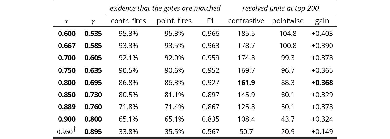
The contrastive advantage persists across the tested matched thresholds. We recomputed the headline top- comparison of Section 5.2 for from to . Because the two gates sit on different scales, we moved both together: each is paired with the pointwise threshold that fires on the closest fraction of the paired elicitations where both gates score the same evidence, and Table 8 reports those firing rates and the overlap of the sets they admit so the pairing can be checked. The contrastive advantage is positive at every threshold, and in every dataset at every threshold (54 of 54 cells). At the reported the matched is ; the paper uses , which fires 4.9 percentage points more often, so the published gain is the more conservative one. Raising alone with fixed at stays positive through and reverses at , where the contrastive gate demands 95 of 100 points on one alternative while the pointwise bar stays below “maybe true”; even at the matched , the two gates admit substantially different sets there (), so we treat that row as exploratory and rest the claim on . We present the matched sweep as a robustness check rather than a preregistered test, since it was designed after the fixed- sensitivity.
We do not treat the 100-point allocations as calibrated probabilities. is a divergence between two distributions over the same alternatives, and “resolved” says that belief has concentrated, not that the leading explanation is 80% likely to be true. What the metric needs is that allocations be stable, insensitive to presentation, and responsive to evidence, which Appendix B, Appendix D, and Appendix J check. We nonetheless compared stated confidence with a reference outside the model. For the 170 directional contrast sets (125 distinct analyses) whose statistic can be recomputed from the raw data, we read off the cell the recomputed statistic implies. On the 166 the method resolves, the leading explanation agrees with that cell on 163 (98.2%) at a mean stated confidence of 0.945, so confidence sits 0.037 below agreement (95% CI to , clustered on the analysis); the gap remains negative after deduplication and leave-one-dataset-out. The top-label expected calibration error is 0.040, and the multiclass Brier score falls from 0.601 for the prior to 0.047 for the posterior. There is no sign of overconfidence against this reference. This check covers the mechanically decidable directional subset, which is easier than the corpus (97.6% of these nodes resolve, against about 83% corpus-wide), and its reference is a significance decision on the same sample; calibration against scientific truth is a separate question.
The thresholds are not arbitrary numerical knobs. The contrastive thresholds are anchored to posterior concentration and normalized information gain. The pointwise thresholds are anchored to the elicitor’s categorical belief scale. The paired calibration then verifies that these two independently motivated threshold systems produce closely aligned decisions on the same evidence, supporting a fair comparison between pointwise and contrastive metrics rather than one driven by mismatched gate strictness.
Following prior work [2], we apply a post-run deduplication pass to test whether a method receives extra credit for repeatedly generating the same semantic hypothesis under different surface forms.
Both pointwise and contrastive runs use the same semantic-equivalence machinery. We first collapse exact-string duplicates, embed the remaining hypothesis texts with the same embedding model, build a Ward agglomerative clustering tree, and use an LLM judge to decide whether proposed cluster merges are semantically equivalent. Each merge decision is judged with votes and accepted only when at least of votes mark the two clusters as the same hypothesis. Thus, both methods use the same embedding model, clustering procedure, judge prompt, judge model, vote count, and merge threshold.
In the pointwise setting, each search node proposes one focal hypothesis. Deduplication is therefore performed at the node level: two nodes are merged if their hypothesis texts express the same claim. This matches the representation used by the pointwise metric, where each candidate is a single hypothesis.
In the contrastive setting, each search node proposes a contrast set containing mutually exclusive hypotheses. Deduplicating only at the node level would be inappropriate: it would treat the whole contrast set as one textual object and would not remove repeated hypotheses across different contrast sets. We therefore flatten contrastive outputs and deduplicate at the hypothesis level. Each hypothesis inside a contrast set is treated as a candidate for cross-node deduplication.
We add one structural constraint: hypotheses from the same contrast set are never merged with each other. They are MECE alternatives to the same analysis question, not replications. For example, “positive effect,” “negative effect,” and “no effect” may be textually related, but they are distinct alternatives by construction. This within-set hard gate prevents deduplication from collapsing valid contrastive alternatives.
We recount the resolved questions of Section 5.2 so that each resolved claim counts once, grouping confirmed pointwise hypotheses and the leading explanations of resolved contrast sets by the clusters above. At , the average number of resolved questions falls from 97.2 to 87.4 for pointwise surprisal and from 161.9 to 141.9 for Contrastive Discovery, so duplicates make up 10.1% and 12.4% of their resolutions, respectively. Contrastive Discovery still resolves 62% more questions than pointwise surprisal, against 67% before deduplication, and leads on all six datasets.
We evaluate our framework on six datasets spanning scientific and social domains, including materials science, astrophysics, finance and policy, software engineering, sociology and labor economics, and online discourse. Table 9 summarizes the datasets used in our experiments, grouping datasets from the same source benchmark where applicable. We then describe dataset-specific caveats and the filtering logic used for the two largest scientific datasets.
| Dataset | Domain | Rows | Cols. | Row unit |
| Materials Project | Materials science | 68,805 | 28 | Inorganic crystal |
| SDSS Galaxy (DR19) | Astronomy | 50,000 | 28 | Galaxy |
| BLADE datasets | ||||
| Mortgage | Finance / policy | 2,380 | 13 | Mortgage application |
| Conversation | Online discourse | 7,975 | 70 | Debate contribution |
| DiscoveryBench datasets | ||||
| Requirements Engineering | Software engineering | 276 | 202 | Survey respondent |
| NLS Raw | Sociology / economics | 12,686 | 61 | Survey respondent |
View original table
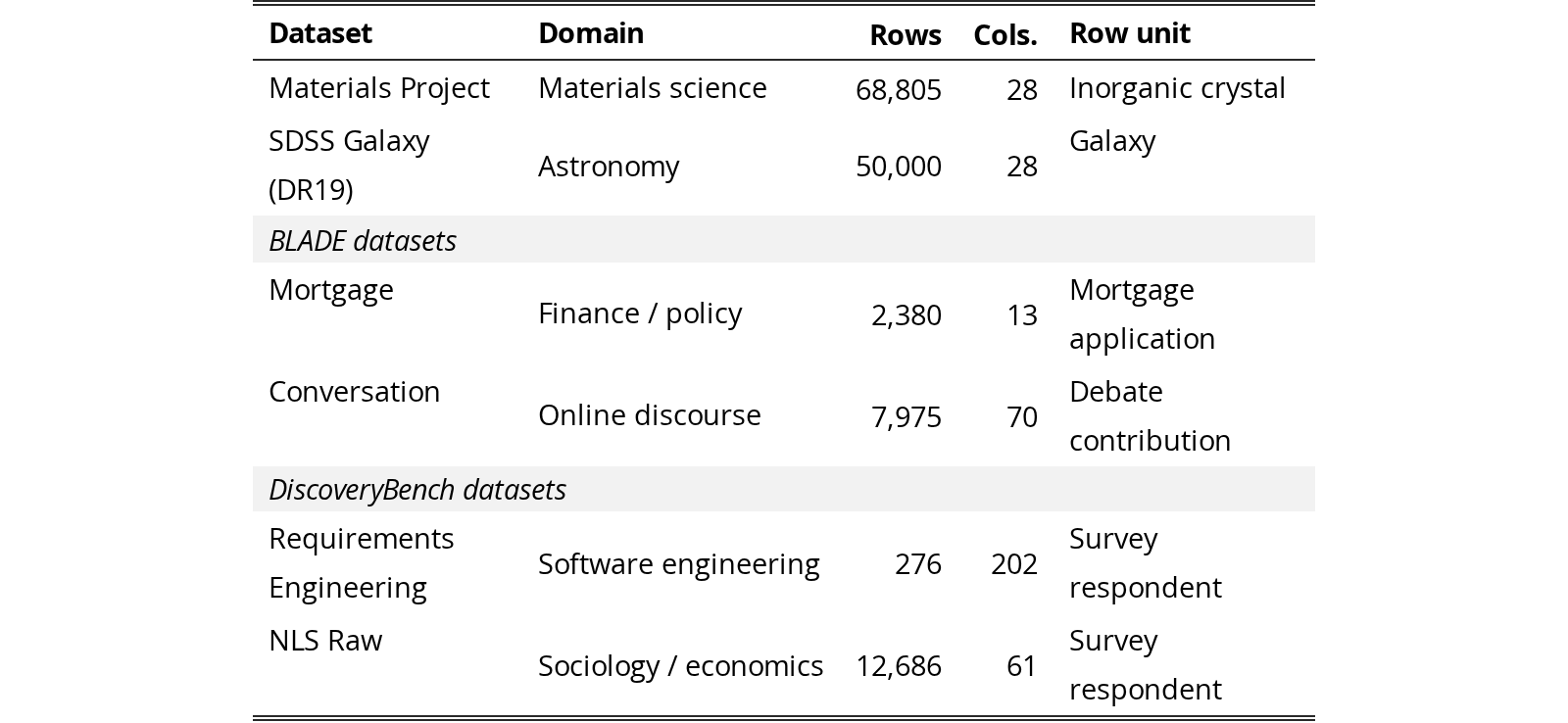
The Materials Project dataset contains 68,805 rows and 28 columns, with each row corresponding to a unique inorganic crystalline material identified by material_id. For our experiments, we restrict the queried subset to materials satisfying nelements , excluding pure elements and materials with five or more constituent elements. We additionally require energy_above_hull eV/atom to focus on near-stable materials. A key caveat is that elastic moduli are missing for approximately 86% of rows; only 9.6K materials have computed elasticity values. Consequently, hypotheses involving elastic properties are evaluated on a self-selected subsample rather than on the full dataset.
The SDSS Galaxy dataset contains 50,000 rows and 28 columns, with each row corresponding to one galaxy identified by a unique specObjID. The dataset represents the astronomy and extragalactic domain. Our query applies the following filters: class = ’GALAXY’, zWarning = 0 to retain clean redshift fits, redshift in the range , and apparent magnitude in the range . The zWarning filter is applied at query time, although the zWarning column itself is not retained in the saved CSV. The query returns the top 50,000 entries under the server-default ordering, which should be interpreted as a minor caveat because the subset is not randomly sampled. Several photometric columns, including modelMag_u, modelMag_g, modelMag_z, petroR50_r, and petroR90_r, use -9999 as a missing-data sentinel. The pipeline does not filter these sentinels. Where we inspected SDSS analyses during the computation audit (Appendix J), the agent’s own code dropped or replaced them before computing statistics. In addition, subClass is missing for approximately 62% of rows.
The BLADE Mortgage dataset contains 2,380 rows and 13 columns, where each row corresponds to one mortgage application. The dataset is situated in the finance and policy domain, with particular relevance to lending and discrimination. Its columns are:
female, black, housing_expense_ratio, self_employed, married, mortgage_credit, consumer_credit, bad_history, PI_ratio, deny, loan_to_value, denied_PMI, accept
Missingness is limited but nonzero: female contains 18 missing values, married contains 2 missing values, and PI_ratio contains 5 missing values.
The BLADE Conversation dataset contains 7,975 rows and 70 columns, with each row corresponding to one contribution, or comment, in an Edge.org debate thread. The dataset belongs to the online discourse and gender participation domain. It contains repeated observations along two axes: 522 unique ThreadId values, with an average of approximately 15 rows per thread and a maximum of 436 rows in a single thread; and 728 unique Id_num contributors, with an average of approximately 11 rows per contributor and a maximum of 504 rows for a single contributor. To avoid contributor leakage, we use an Id_num-level split: 70% of contributors are assigned to discovery and 30% to validation. This preserves row-level granularity while preventing contributor-specific attributes from leaking across splits. We prioritize contributor-level splitting because the contributor axis contains more invariant attributes, including gender, PhD institution, and h-index.
The DiscoveryBench Requirements Engineering dataset contains 276 rows and 202 columns, with each row corresponding to a unique survey respondent identified by ID. The dataset belongs to the software engineering domain and captures practices in requirements engineering for ML-enabled systems. Because the dataset has only 276 respondents, it has limited statistical power for detecting subtle effects. In addition, many of the 202 columns are binary indicators derived from multi-select survey questions, which should be considered when interpreting hypotheses involving sparse or highly correlated features.
The DiscoveryBench NLS Raw dataset contains 12,686 rows and 61 columns, with each row corresponding to a unique NLSY79 survey respondent identified by ID. The longitudinal panel has already been flattened into a wide-format representation with one row per person. The dataset is situated in the sociology and labor economics domain. A key caveat is that columns mix measurements from different survey years, including 1979, 1981, and later waves. Therefore, hypotheses over this dataset should respect the implicit temporal ordering of variables and avoid treating later measurements as valid predictors of earlier outcomes.
For the two large scientific datasets, Materials Project and SDSS Galaxy, we apply simple domain-motivated filters before running hypothesis generation. These filters are not intended to optimize downstream performance. Instead, they define physically coherent, cleanly measured, and computationally tractable hypothesis spaces. In both cases, the goal is to avoid forcing the model to generate hypotheses across incompatible physical regimes or over measurements known to be unreliable.
For SDSS Galaxy, we restrict the dataset to entries with class = ’GALAXY’. This keeps the hypothesis space physically coherent: stars, quasars, and galaxies obey different physical regimes, and several galaxy-oriented columns, such as size and profile-radius measurements, would be meaningless or differently interpreted for non-galaxy objects. We also require zWarning = 0, the standard SDSS quality flag indicating a clean redshift fit. Nonzero warning values often indicate failed pipeline checks, such as low signal-to-noise, bad template matches, or problematic spectra; including these entries would inject unreliable redshift-dependent measurements into many hypotheses.
We further restrict redshift to . The lower bound removes very nearby objects for which peculiar velocities can be comparable to the Hubble-flow velocity, making redshift a poor distance proxy. The upper bound keeps the sample within the approximate regime of the SDSS Main Galaxy Sample, rather than mixing in higher-redshift luminous red galaxies or other populations governed by different selection effects. Finally, we require . The bright-end cut avoids saturated sources for which photometry may be unreliable, while the faint-end cut avoids objects for which photometric uncertainty and redshift signal-to-noise become limiting. The top-50,000 cap is a practical scale constraint: it remains below the SDSS unauthenticated query limit, fits comfortably in memory, and provides sufficient statistical power for hypothesis generation. Unlike the physical and quality filters, this cap is primarily pragmatic rather than physically principled.
For Materials Project, we restrict to materials with nelements . This excludes pure elements, whose small and heavily studied set would make many property hypotheses trivial or degenerate. It also excludes materials with five or more elements, such as high-entropy alloys and complex multicomponent oxides, where individual elemental contributions are often highly entangled and harder to interpret cleanly. Retaining binary, ternary, and quaternary compounds captures much of functional inorganic chemistry, including families such as rock salts, perovskites, spinels, and Heusler compounds, while keeping the hypothesis space tractable.
We additionally require energy_above_hull eV/atom. This threshold follows the common Materials Project convention for selecting materials that are plausibly synthesizable or near-stable. Materials substantially above the convex hull are increasingly likely to be hypothetical or physically unstable, making their computed properties less useful for generating hypotheses about realizable materials. This filter also removes unusual metastable phases whose extreme properties could dominate regressions or produce hypotheses driven by outliers rather than robust physical structure.
Across both scientific datasets, the filters are chosen to satisfy four criteria. First, retained samples should be physically coherent, so that hypotheses are generated within a comparable regime. Second, measurements should be clean enough to avoid obvious garbage-in, garbage-out effects, such as failed redshift fits or saturated photometry. Third, the filtered datasets should remain large enough to support statistically meaningful hypothesis generation. Finally, the filters should be conventional enough to be defensible to domain experts, rather than appearing as post hoc cherry-picking.
The resulting benchmark portfolio covers six domains: materials science through Materials Project, astrophysics through SDSS Galaxy, finance and policy through BLADE Mortgage, software engineering through DiscoveryBench Requirements Engineering, sociology and labor economics through DiscoveryBench NLS Raw, and online discourse through BLADE Conversation. The datasets also span a broad range of sample sizes: 276 rows for DiscoveryBench Requirements Engineering, 2,380 rows for BLADE Mortgage, 7,975 rows for BLADE Conversation, 12,686 rows for DiscoveryBench NLS Raw, 50,000 rows for SDSS Galaxy, and 68,805 rows for Materials Project. This row-count spread is useful for analyzing how hypothesis-generation and validation behavior vary under different statistical-power regimes.
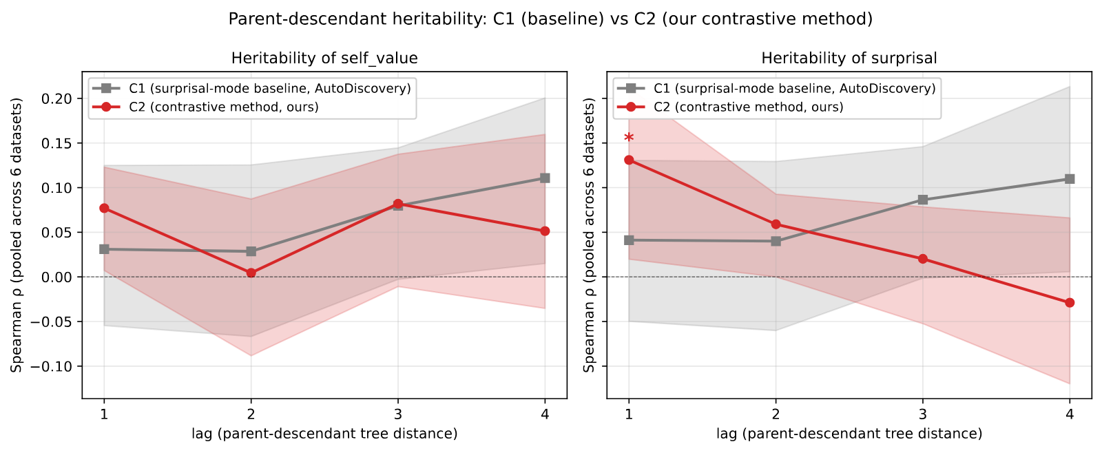
A precondition for hierarchical MCTS to outperform flat sampling is that ancestor scores predict descendant scores. Without such correlation, UCT’s value-back-propagation has nothing to exploit when choosing which subtree to expand, and the selection rule is statistically equivalent to uniform-random parent selection. To test whether this property holds in our setting, we measured the parent–child Spearman rank correlation of self_value (the scalar UCT propagates) across the 200 experimental validations of each search tree, pooled across six datasets. We use self_value as the headline metric because it is what UCT directly reads when computing -values. As a robustness check we additionally report the underlying surprisal (the logged belief change: in the surprisal-mode baseline, in the contrastive method), which has none of the clipping or -normalization construction in self_value. For the contrastive method this secondary quantity is the entropy reduction logged as a diagnostic alongside each node, not the contrastive belief shift of Section 3.3; self_value is the clipped that UCT reads. Reporting both addresses the concern that an observed parent–child correlation could be a construction artifact rather than a real property of the search tree.
The surprisal-mode baseline (pointwise) yields essentially zero parent–child heritability at lag 1 (, 95% CI , pairs, BH-FDR ): UCT-driven selection in this regime operates without exploitable score signal. Our contrastive partition reward (Contrastive) shows a positive lag-1 trend (, 95% CI , , raw permutation ) that is not significant after Benjamini–Hochberg correction across the 7-lag family () but FDR-significant on the underlying surprisal score (, ). The Contrastive trend on surprisal decays monotonically toward zero by lag 4, consistent with local inheritance. The baseline shows no such decay structure on either metric. See Figure 6.
We note that the Contrastive correlation is consistent with two mechanisms our analysis cannot uniquely distinguish: (a) inheritable signal in the score itself, exploitable by UCT-selection; or (b) a downstream effect of the structured -cell partition being available as ancestor context to the next-level proposer, which would correlate child and parent scores through generation rather than through selection. The natural ablation, comparing UCT-selection to uniform-random parent selection while preserving context inheritance, would adjudicate (a) vs. (b) and is left to future work.
This appendix gives the protocol, reliability, and control analyses behind Table 1.
Thirty-eight evaluators with MS or PhD degrees in the mathematical, computational, or natural sciences, recruited and screened separately from the authors (31 through a screened crowd platform, 7 verified in person), rated 60 blinded items: ten per dataset, stratified by the contrastive score . Each evaluator saw only the research question, the candidate explanations, and the statistical evidence from the executed analysis, with the alternatives in random order; our system’s beliefs, its resolution label, and the pointwise verdict were never shown. Each item was rated by at least 4 evaluators (median 8). The four questions per item were (Q1) which explanation the evidence supports, with the extra options “none of these is supported” and “cannot tell”; (Q2) whether the alternatives are mutually exclusive and cover the plausible explanations, with options for a missing explanation, overlap, or both; (Q3) whether the result is worth reporting; and (Q4) whether the chosen variables and test fit the question. We score items by majority vote and count no majority, “cannot tell,” and “none” as disagreement with our system’s explanation. Five submissions were excluded under a rule fixed at the first exclusion (one incomplete session and four evaluators who missed both attention checks). Restricting to the 30 evaluators who caught every attention check lowers the overall agreement from 71.7% to 68.3%, so inattentive raters do not carry the result. Expert evaluations were collected with informed consent and kept confidential; the information concerned our methods and scientific outputs, not the evaluators as individuals. Under our institution’s IRB guidance, this activity does not constitute human-subjects research and therefore did not require IRB review.
Both methods were compared on the same 60 questions, using the same evidence and expert judgments. The pointwise hypothesis was the explanation our system rated most plausible before seeing the evidence, evaluated on its own.
The expert majority matched our system’s explanation on 43 of 60 items (71.7%, 95% CI 60.0–83.3 by item-clustered bootstrap): 40 of the 51 items it marked resolved (78.4%) and 3 of the 9 it left unresolved. Of the 17 disagreements, the experts chose a competing explanation on only 3; on 8 they judged the evidence insufficient and on 6 they formed no majority, so most disagreements fall on evidence the experts themselves could not settle. Across all 60 items the panel committed to a specific alternative on 46, which shows that the executed experiments usually separate the alternatives well enough for experts to commit. Agreement was 79% on confirmative resolutions and 77% on corrective ones. Against the pointwise baseline: on the 32 items it confirmed, the experts endorsed 23 findings for each method; on the 22 items it rejected and stopped, the alternative our system identified matched the expert majority on 18 (81.8%; exact 95% CI 60–95). A related subset, the 22 items the baseline did not confirm and our system resolved, overlaps this one on 19 items and gives 17 of 22; the main text reports the pointwise-rejected subset. Per dataset, agreement ranges from 6 of 10 to 9 of 10, too few items to compare domains.
On the load-bearing judgment (Q1, four to six options), pairwise agreement was 64% and Krippendorff’s was 0.54 (95% CI 0.45–0.61), and in a descriptive stratification was 0.60 on resolved items versus 0.22 on unresolved ones, so rater disagreement concentrates on the items Contrastive Discovery leaves unresolved. On set completeness (Q2), 80% of ratings judged the set well formed, 15% flagged a missing plausible alternative, 4% overlap, and 1% both; raw agreement on the binary omission call was 83% (Gwet’s AC1 ; the lower Fleiss’ of 0.35 reflects the 80/20 response skew). A strict majority flagged a missing alternative on 6 of the 60 sets. Analysis appropriateness (Q4) was judged appropriate on 73% of ratings, wrong variable or test on 19%, and cannot tell on 8% (binary raw agreement 72%, AC1 ). Scientific value (Q3) had low agreement (), so we report it only as a distribution: 51% substantive finding, 20% minor, 3% too obvious to state, 25% not a finding.
To check that the ratings track genuine quality, we planted two manually constructed defective sets among the items, one with a plausible alternative removed and one with overlapping alternatives: 11 of the 14 evaluators who saw the first flagged a missing alternative and none confused it with overlap, and 10 of 12 flagged the second as defective. On separate control items we kept the contrast set intact but paired it with the evidence of a different question: the well-formed rate stayed at 77%, close to its 80% baseline, while the analysis-appropriateness rating fell from 73% to 7% and the wrong-variable-or-test flag rose from 19% to 84%. The evaluators therefore flag real set defects without blanket-flagging, and recognize when an analysis does not fit its question. Attention controls (mismatched evidence expected to yield “cannot tell”) fired as expected on 95% of exposures.
The experts read the same evidence as our system, so their agreement shows that resolutions track the evidence as independent experts read it; it is not a test of scientific truth. The experts were general quantitative-science raters rather than specialists matched to each item’s subfield, and they judged the executed analysis rather than replicating it. The comparison with the pointwise baseline is one of endorsed yield, not of accuracy on the items both methods decide.
The belief step reads the analyst’s written summary of an executed analysis. Three audits, none of which involves a language model in the scoring, check that this chain is faithful: that the adjudication follows the evidence it is shown, that the summary reports the numbers the code printed, and that the code computed those numbers correctly.
We took 14 claims from 10 DiscoveryBench training questions with documented findings (a finding with two claims contributes two), constructed contrast sets whose wording was held fixed across conditions, and ran the production posterior elicitor (gpt-4o-2024-08-06, five samples, ) on numbers-only evidence with the alternatives in randomized order and no analyst prose. Given the full statistic with its interval, available for 11 of the 14, the elicitor placed the documented answer first in every case and resolved 8 of 11, holding back on three whose intervals lie close to zero. Given the coefficient without an interval it still ranked the documented answer first on 13 of 14 while resolving only 7, appropriate caution when the evidence is incomplete. In a separate condition covering all 14 claims, we supplied the statistic with its sign reversed; the resolution followed the reversal in every case. Supplying no evidence produced no resolution on any of the 14 (largest posterior 0.74). Because the wording of the alternatives was identical across the four conditions, these resolutions follow the evidence and not the phrasing. This establishes evidence-driven adjudication, not end-to-end correctness of the pipeline that produces the evidence.
Across all available seeds, 3,015 analyses contained checkable numerical claims in the analyst’s written summary. We checked, allowing for rounding, percentages, and scientific notation, whether those numbers appear in the captured standard output of the executed code. 99.1% of these analyses and 99.7% of the 9,239 checked numbers are grounded in a printed value. Reading every mismatch by hand found at least five genuine slips, including a slope quoted from a plot-only run and a count reported as a percentage; the audit caught all of them without a human in the loop. Pairing each summary with a different analysis’s output and re-running the identical matcher grounds only 3.8% of numbers, so the check discriminates. Signs are not checked by this audit.
For the analyses whose statistic can be rebuilt directly from named columns of the raw data (400 of 3,274; 331 scorable, spanning every available seed and 251 distinct dataset/test/column combinations), we recomputed the statistic with standard libraries and compared it to the value the agent printed. The values matched on 318 of 331 (96.1%). Every mismatch we could trace came from our recomputation missing a data-handling step in the agent’s code (a custom parser, a missing-data rule, a sentinel replaced before analysis, a group split); a few could not be classified either way. We found no confirmed computation error. Substituting a wrong column matches only 2.1% of the time, so the check is not loose. Coverage is 12% of analyses and not random, since the rebuildable analyses are the simpler ones, so we read this as a check on the covered analyses rather than a pipeline-wide rate.
A contrast set that omits the explanation the evidence supports can produce a confident wrong resolution. We measured how often this happens and how well the abstention alternative of Section 3.4 prevents it.
We used two frozen panels. The primary panel is 163 questions, all directional triples (), whose supported explanation is fixed by a statistic recomputed from the raw data with no model in the scoring (121 distinct underlying analyses; intervals are clustered on the analysis). Because the correct answer must be present to be removed, this panel conditions on questions the system originally resolved correctly, so the intact-set control measures re-elicitation stability rather than corpus accuracy. A secondary panel is 40 resolved questions across six partition types and whose supported explanation matches the blinded expert majority of Appendix I. The design crossed two factors: the set as generated or with the supported explanation removed, each with or without an added alternative worded “none of the listed alternatives matches the evidence; the contrast set is incomplete.” The seven secondary-panel questions with omitted the removed-explanation condition without the added alternative, since its sole survivor would receive all belief by construction. Selecting the added alternative flags the set as incomplete; declining to reach withholds resolution as before. Cell order was randomized per call and five samples were requested for aggregation before thresholding. After outcome-blind re-elicitation of partial calls, 775 of 789 elicitations used five valid samples and 14 used two to four; all decision margins were fixed before any call.
| of which resolved to | ||||
|---|---|---|---|---|
| Supported explanation removed | Declined or flagged | Unsupported | no effect | competing direction |
| Contrast set as generated | 46.6% | 53.4% | 50.9% | 2.5% |
| With “none of the above” | 99.4% | 0.6% | 0% | 0.6% |
View original table

With the sets left intact, the supported explanation resolved on 159 of 163 questions (97.5%) without the abstention alternative and on 162 of 163 (99.4%) with it, and the abstention alternative was never selected (0 of 163). With the supported explanation removed (Table 10), the system resolved to a surviving alternative on 53.4% of questions, so an omitted explanation can indeed produce a wrong resolution. The failures lean toward caution: when a direction was removed and the null survived, the system resolved to “no detectable effect” on 58.5% of cases, left the question unresolved on 38.7%, and asserted the opposite direction on 2.8%; when the null was removed and only opposing directions survived, it left all 21 unresolved. Those null resolutions are still wrong under our reference, which is why the abstention alternative matters. The abstention alternative cuts false resolution to 0.6%: it is the leading option on 92.6% of removed cases (mean mass 0.85) and crosses the 0.80 threshold on 69.3%, identifying the omission rather than only withholding an answer. The secondary panel shows the same pattern with wider intervals (63.6% false resolution without the option, 6.1% with it, on the 33 questions with ). The discovery runs of Section 5.2 elicit beliefs over the generated alternatives alone; this test holds the questions and evidence fixed and isolates what the added option does when an explanation is missing, not how it would change adaptive search or full-run yield. In those runs a missing alternative can force a wrong resolution only on a set that omits one, and two external checks show such sets are few: a strict majority of experts flagged a missing alternative on 6 of the 60 sets they rated, and on the 51 items our system resolved, experts preferred a competing explanation on only 1 (Appendix I).
This appendix gives the details behind Section 5.5. All analyses replay or re-score the logged discovery runs; none changes the resolution rules or the aggregation of the headline (within-run top-, seed mean within dataset, then mean over the six datasets).
Every run logs the cost of each individual candidate. Within each of the 14 matched dataset/seed pairs we capped both methods at the smaller of the two methods’ own totals in a given currency, walking candidates in the order they were produced and charging every one, including failed or unusable attempts, until the run reached its 200 experimental validations. Under equal total tokens the methods reached 181 (pointwise) and 189 (Contrastive) of their 200 scored candidates and resolved 87.7 against 148.3 units (difference , 95% interval over six dataset clusters ); under equal logged dollars, 92.2 against 145.8 (); charging output tokens only, 95.8 against 124.9 (, the one interval that includes zero; five of six datasets positive). Applying one common budget to every run (4.45M tokens, the smallest total that any run spent) gives 52.4 against 89.6. Belief elicitation accounts for 8.5% of contrastive tokens against 2.5% for pointwise, but total spend per candidate is similar (61.1k tokens for pointwise against 52.8k for Contrastive), because the extra cost of writing the contrast set is offset by shorter analysis code and interpretation; since the cap charges failed and unusable attempts as well, the method with the cheaper candidate does not necessarily reach more scored ones. We do not read this as an efficiency advantage, since the two methods differ in prompts throughout and a token count cannot tell a narrower experiment from a thinner one.
Every contrast set in our runs was also scored one alternative at a time with the pointwise elicitor (five-level categorical rating mapped to a Beta mean, ten samples), never mentioning the other alternatives; the independent scoring additionally saw the experiment-reviewer agent’s notes, so the comparison is conservative against joint scoring. Applying the pointwise method’s own gate () to the independent scores under the paper’s estimator gives 157.8 resolved units at top-200 when exactly one alternative passes (165.4 when any passes), against 161.9 for joint scoring: a difference of 4.1 units, about 6% of the 64.7-unit headline gap, with a interval that includes zero. The two scorings name the same leading alternative on 89.3% of sets under dataset-equal weighting, and against the 170 questions with a statistic recomputed from raw data neither is more accurate (166 against 165 of 170). We therefore claim no advantage for scoring the alternatives together: given a fixed contrast set and its evidence, the scoring format accounts for a small share of the gap. Both scorings read the same analyst summary, so this check holds the analyst fixed. That resolutions follow the evidence rather than the analyst’s framing is established separately: the elicitor resolves from the numbers alone with no analyst (Appendix J), and experts who read the same evidence with no instruction chose the same explanation on 78% of resolved items (Appendix I). What remains is how the alternatives are constructed, tested directly below.
Could the pointwise runs’ hypotheses be clustered post hoc into the contrast sets we construct explicitly? Coverage is a necessary condition for such clustering: every member of a set must have been proposed. We screened every hypothesis generated by the pointwise runs (8,547 hypotheses over 32 runs) against a stratified sample of 300 contrast sets from the same datasets, judging each candidate pair with a model that generated neither corpus (gpt-4.1-mini) under a rubric that permits refusal. The matcher assigns a set’s own alternatives to the correct member on 99.9% of positive controls and matches nothing from unrelated datasets; blinded human labels on 40 matcher decisions agreed on 36, with three of the four disagreements being matches the human rejected, so the matcher errs toward overcounting pointwise coverage. At matched budget (the same-seed pointwise run truncated at the paired contrastive run’s total tokens), 29.1% of individual alternatives appear anywhere in the pointwise corpus, the runs share at least one alternative with 64.7% of the sets, and the complete set is present for 2.6% of the questions that at least one pointwise hypothesis addresses (95% interval , truncated at zero). Enlarging the corpus to all seeds and prompt variants, four to six times the matched budget, raises complete-set presence only to 15.4% (, wide) and per-alternative coverage to 53.7%. The explanation that the evidence eventually supports is present 52.0% of the time when it confirms the prior-leading explanation but 25.4% when it corrects it (paired difference percentage points, ), so exactly where pointwise evaluation rejects its hypothesis and stops, its corpus usually lacks the explanation that turns out to hold.
Stratifying the frozen top-200 pool of Section 5.2 by contrast-set size, resolution is 93.4% with two alternatives (102 questions, 4.4% of validations, dataset-weighted), 83.2% with three (2,217; 78.3%), and 68.3% with four (479; 17.3%). Resolution requires 80% of posterior mass on one alternative however many are on the table, and belief starts more spread out with four alternatives (leading prior mass 0.41) than with two (0.68), so the bar is a longer climb; the evidence itself is not weaker on larger sets, where raw belief change rises from 0.59 to 1.07 bits. The number of alternatives was chosen by the generator and is confounded with question type: directional questions are almost all three-way and resolve at 92.7%, and a separate pooled comparison gives a three-to-four gap of 15.7 percentage points, which shrinks to 2.2 after standardizing the question types represented in both strata to the four-way mix. On paired support-scope questions the pointwise gate fires 12.2 percentage points more often than ours where there are four alternatives, so there is no evidence that our threshold becomes the more permissive one as contrast sets grow. This series covers two to four alternatives, excluding one five-way and one seven-way question, and describes how resolution varies with ; it does not isolate a causal effect of .
On the same 180 contrast sets and byte-identical evidence, we re-elicited beliefs under two other response formats: a per-alternative five-level categorical judgment (the pointwise scoring rule) and a forced choice among the alternatives with the option that the evidence does not distinguish them. Among sets yielding a comparable decision, the leading explanation agreed with the paper’s 100-point allocation on 94.2% of sets under the categorical format (161 of 171) and 99.3% under forced choice (152 of 153), against 98.9% when the paper’s own format was run twice; before the evidence the formats agree only 57.1% and 76.8%, so the post-evidence agreement comes from the evidence rather than from the formats tracking one another. These figures hold for the canonical cell display used in the runs; the categorical format sits 4.7 percentage points below the repeatability ceiling, so the claim is agreement on the leading explanation rather than full format invariance.
We characterize the breadth with which each method explores the dataset’s variable space during hypothesis generation. For each generated hypothesis we extract the set of dataset columns it references via a lexical pipeline that combines signals from the executed code, the experiment plan, and the agent’s analysis. Letting denote the canonical columns referenced by hypothesis and the dataset’s total column count, we define cumulative column coverage and summarize each trajectory with a two-parameter saturating-exponential fit , where is the asymptotic coverage fraction and is the rate constant; this is the rank-1 summary of a biased coupon-collector process in which high-salience columns are sampled more frequently than low-salience ones.
Figure 7, Figure 8 and Table 11 report the fits across our six datasets. On four of six datasets both methods reach high asymptotic coverage (), and pointwise reaches a higher asymptote than Contrastive on five of six. Requirements Engineering has the lowest coverage, with fitted asymptotes of for pointwise and for Contrastive: about half of its columns are never touched by either method, however many hypotheses are proposed. Figure 9 and Table 12 compare column overlap between sibling and non-sibling nodes.
| Pointwise | Contrastive | ||||||
|---|---|---|---|---|---|---|---|
| Dataset | |||||||
| Materials Project | 28 | 0.955 | 0.056 | 157 | 0.919 | 0.062 | – |
| BLADE Conversation | 70 | 0.905 | 0.033 | – | 0.863 | 0.038 | – |
| Requirements Engineering | 202 | 0.513 | 0.015 | – | 0.411 | 0.015 | – |
| SDSS Galaxy | 28 | 0.955 | 0.103 | 87 | 0.955 | 0.065 | 176 |
| BLADE Mortgage | 13 | 1.000 | 0.290 | 11 | 0.999 | 0.274 | 11 |
| NLS Raw | 61 | 0.974 | 0.036 | 139 | 0.909 | 0.027 | – |
View original table
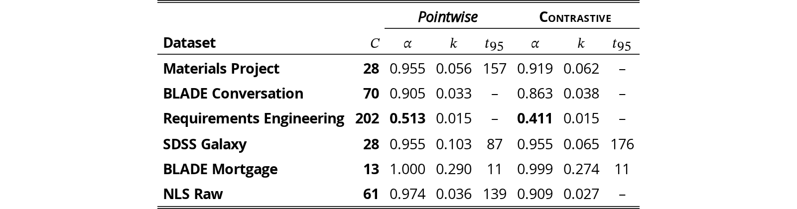
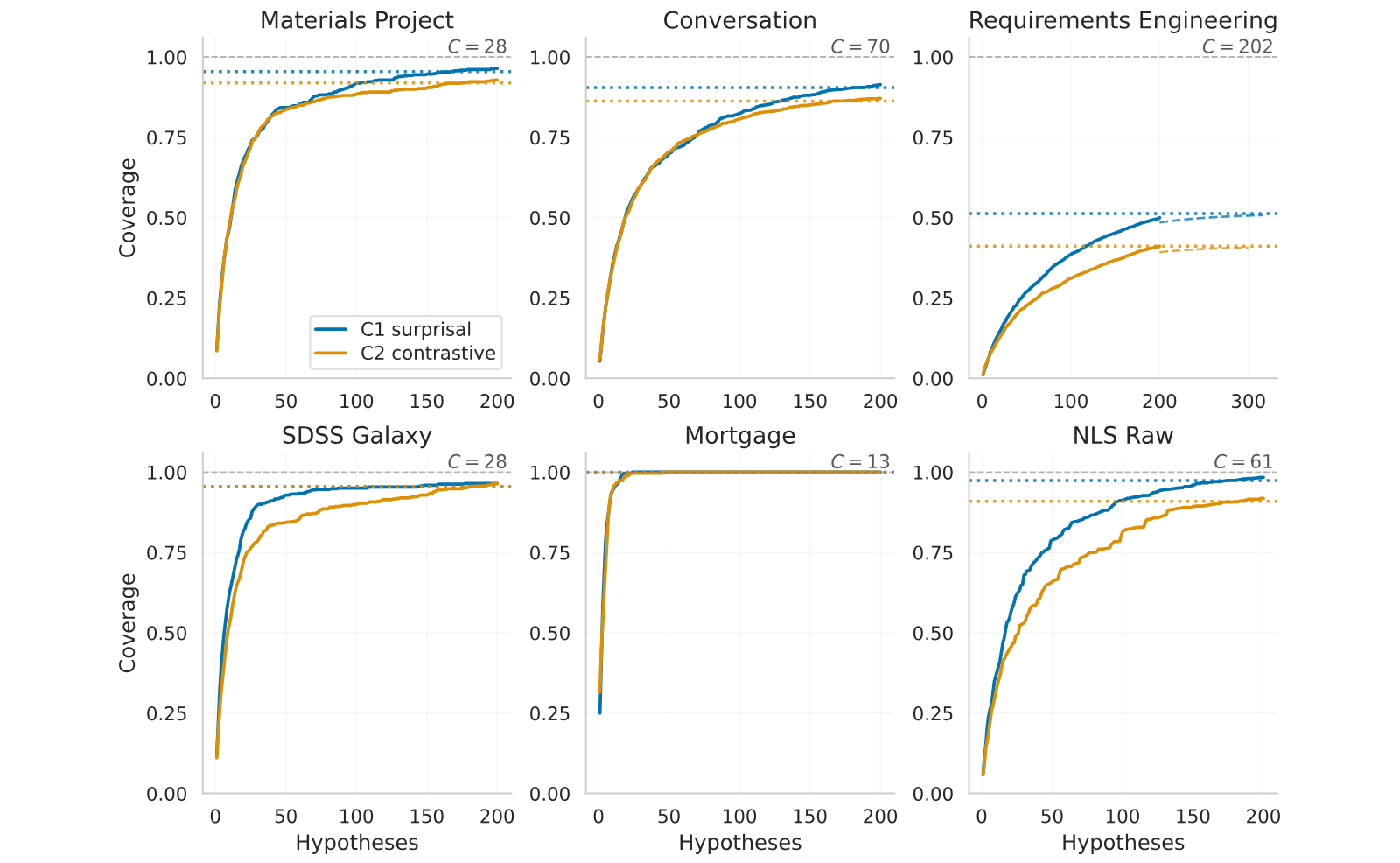
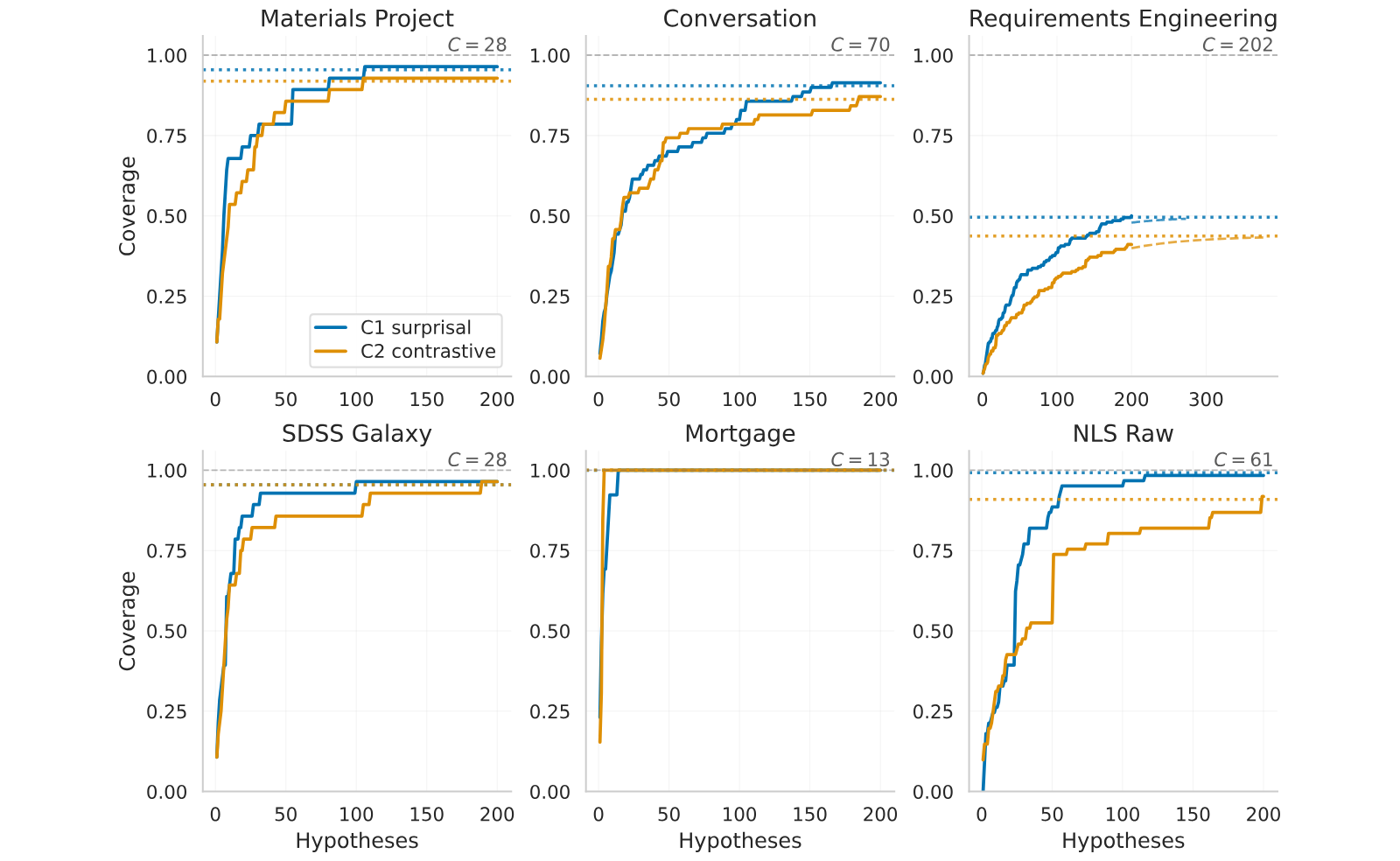

| Pointwise | Contrastive | |||||||
|---|---|---|---|---|---|---|---|---|
| Dataset | ||||||||
| Materials Project | 2.43 | 0.031 | 0.094 | 0.135 | 2.45 | 0.064 | 0.092 | 0.130 |
| BLADE Conversation | 4.06 | 0.048 | 0.074 | 0.320 | 4.20 | 0.097 | 0.085 | 0.305 |
| Requirements Engineering | 2.41 | 0.023 | 0.024 | 0.505 | 2.34 | 0.135 | 0.080 | 0.415 |
| SDSS Galaxy | 3.41 | 0.089 | 0.113 | 0.135 | 3.21 | 0.150 | 0.135 | 0.135 |
| BLADE Mortgage | 3.71 | 0.170 | 0.211 | 0.065 | 3.93 | 0.235 | 0.255 | 0.065 |
| NLS Raw | 4.68 | 0.075 | 0.090 | 0.300 | 3.39 | 0.059 | 0.077 | 0.280 |
View original table
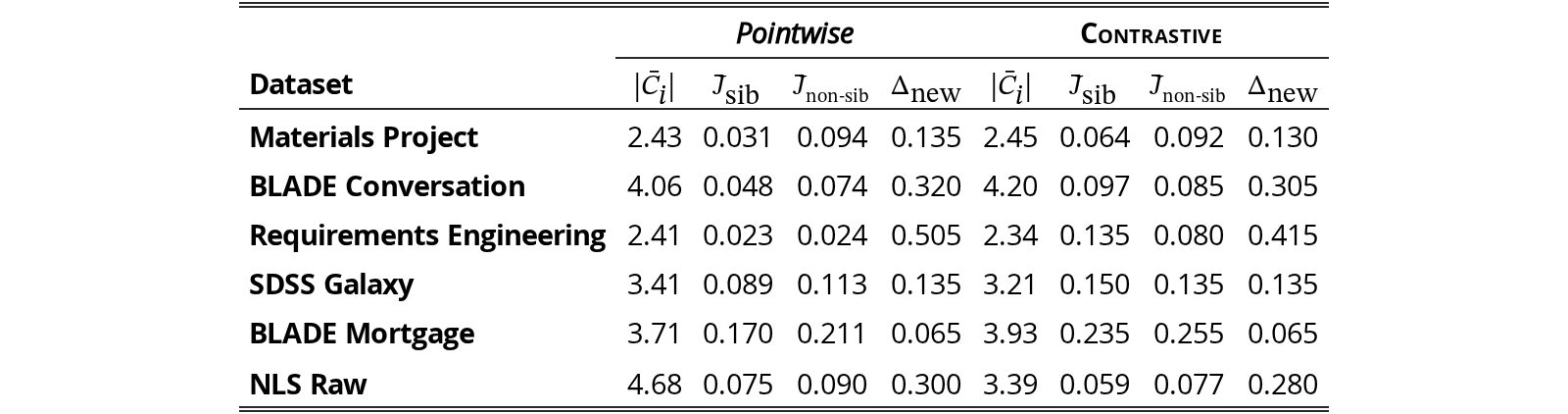
For each generated hypothesis, we extract the set of dataset columns it references by parsing four fields from the run logs: the hypothesis text, the agent’s experiment plan (objective, steps, deliverables), the executed Python code, and the agent’s textual analysis. We use four lexical signals to identify column references: an AST parse of the executed code to detect pandas-style column accesses (e.g., df[’col’]), a regex fallback for cases where the code fails to parse, identifier tokenization on statsmodels-style formula strings, and substring matching of canonical column names against the concatenated textual fields. Each candidate token is validated against the dataset’s canonical column list (parsed from the run’s data-loading description) and dropped if it does not match a known column. The pipeline is fully lexical and uses no LLM calls.
Given per-hypothesis touched-sets for a single run of hypotheses, we define cumulative coverage as
where is the dataset’s column count. We summarize each trajectory with a two-parameter saturating exponential fit
where is the asymptotic coverage fraction and is the rate constant. Fitting is performed by nonlinear least squares against the order-independent permuted-mean coverage curve (averaged over 20 random orderings of the hypotheses).
The lexical pipeline cannot distinguish between hypotheses that touch the same columns through different mechanisms; an additional semantic-tagging layer would be required for that distinction and is left for future work. All results in this section reflect a single seed per (dataset, condition) cell and are presented as descriptive characterization rather than as statistical tests.
We screened 14 questions with published findings from the DiscoveryBench [32] training split and tested recovery on ten leakage-screened questions (questions whose wording gives away the answer were excluded). Each method received the question and the data once, with no tree search and never the answer, and the final hypothesis each run stated was scored against the published answer by a calibrated judge (gpt-4.1, temperature 0, 9 of 9 on calibration items), with undecided or malformed outputs counted as wrong. Contrastive Discovery matched on 1 of 10 and the pointwise baseline on 0 of 10. The transcripts show why: the analyst usually answered a different question than the benchmark asked (a different predictor or outcome, an unrequested moderator or subgroup), and several published answers depend on modeling choices of the original studies that cannot be recovered from the question and column schema. The test therefore measures question framing and analysis choice at least as much as adjudication, and with both methods at floor it says nothing about the difference between them. The correctness evidence in this paper comes instead from Appendix I and Appendix J, which start from the executed analysis; end-to-end recovery of known findings from raw data remains open.
The pointwise and Contrastive methods share the discovery scaffold but differ in how beliefs are elicited and in what the analyst is asked to report. We list the main differences here, with what has been tested about each.
- •
Response format and aggregation. Pointwise beliefs are five-level categorical ratings (ten samples) mapped to a Beta mean (Appendix ); Contrastive beliefs are 100-point constant-sum allocations (five samples) averaged into a distribution (Appendix ). Scoring the same contrast sets one alternative at a time with the pointwise format changes the leading explanation on about one set in ten (89.3% agreement) and the headline by 4.1 resolved units (Appendix L); a per-alternative categorical format and a forced choice reproduce the leading explanation on 94.2% and 99.3% of sets yielding comparable decisions (Appendix L).
- •
Elicitor instructions. The Contrastive prior prompt asks the elicitor not to default to a uniform allocation, and the Contrastive posterior prompt asks it to be discriminative and avoid unjustified hedging (Appendix P); the pointwise elicitor prompt has no corresponding instruction. Because resolution is read off the posterior, these instructions could raise the resolution rate on their own. Two checks bound this. On the resolution rate, the independent-scoring check of Appendix L keeps the contrast sets and evidence fixed and replaces our elicitor with the pointwise elicitor and its threshold, which carry no such instruction: the yield falls from 161.9 to 157.8 questions, about 4 of the 64.7 gained over pointwise. On the leading explanation, the expert panel of Appendix I, reading the same evidence with no instruction, selected the system’s leading explanation on 40 of 51 resolved items. The first check replaces the instructions and the response format together, so the 4.1 questions bound their combined effect. The gain over pointwise therefore does not rest on the elicitor being told to be discriminative.
- •
What the analyst reports. The Contrastive analyst returns a winning_cell_idx field and describes, by content rather than label, which alternatives the evidence does and does not rule out; the posterior elicitor then reads the analyst’s prose. The pointwise analyst writes a free summary of the code output. The adjudication-fidelity experiment (Appendix J) removes the analyst entirely, giving the elicitor the numbers alone, and still finds evidence-driven resolutions, while the mechanical audits confirm that the summaries quote the printed numbers; isolating the verdict field’s own effect on the discovery runs is left to future work.
- •
When alternatives are generated. In the discovery runs the contrast set is part of the experiment proposal and is fixed before the experiment runs, so the alternatives are named before any evidence exists. The post-hoc companion of Section 5.1 generates its alternatives from the hypothesis under test, the dataset’s variables, and the same earlier context a live proposer would have; the current analysis, its output, and the verdict on the hypothesis are withheld, and the companion is applied whether the hypothesis was confirmed or rejected.
- •
Review and revision. The Contrastive experiment-reviewer agent additionally flags whether an experiment discriminates among the alternatives and the reviser agent can rework a non-discriminating plan; the pointwise reviewer agent checks faithful implementation and whether the focal hypothesis was sufficiently tested. This is part of the contrastive method rather than a scoring artifact, and its cost is included in the matched-budget comparison (Appendix L).
- •
Normalization. Pointwise surprisal is normalized by an achievable ceiling derived from the prior (Appendix ), whereas is scaled by the constant (Appendix ); the consequences of each are discussed where they are defined.
Refer to Figure 10, Figure 11, and Figure 12 for a per-dataset breakdown. Counts are averaged over runs, so the under each dataset is the mean number of nodes per run, shown to one decimal where the mean is fractional; the pooled column sums the six per-dataset means.
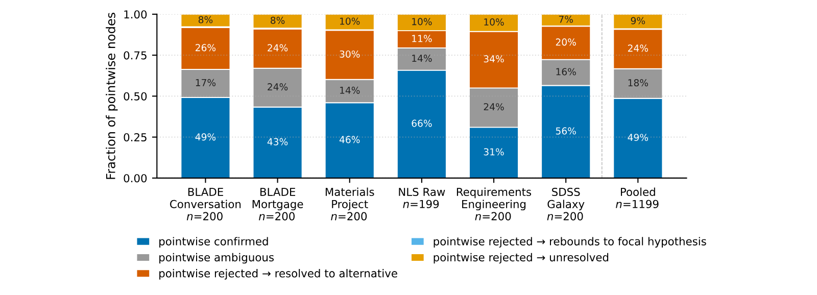
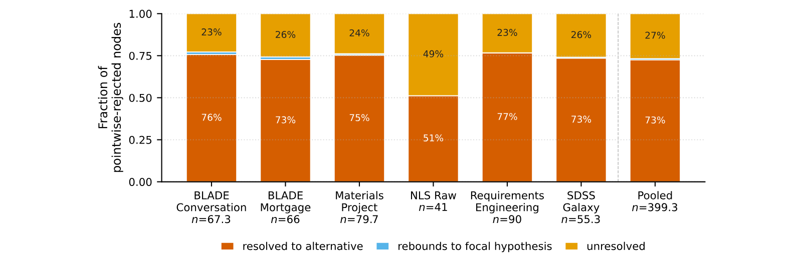
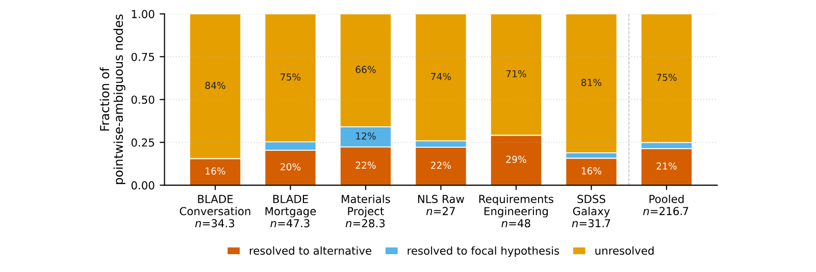
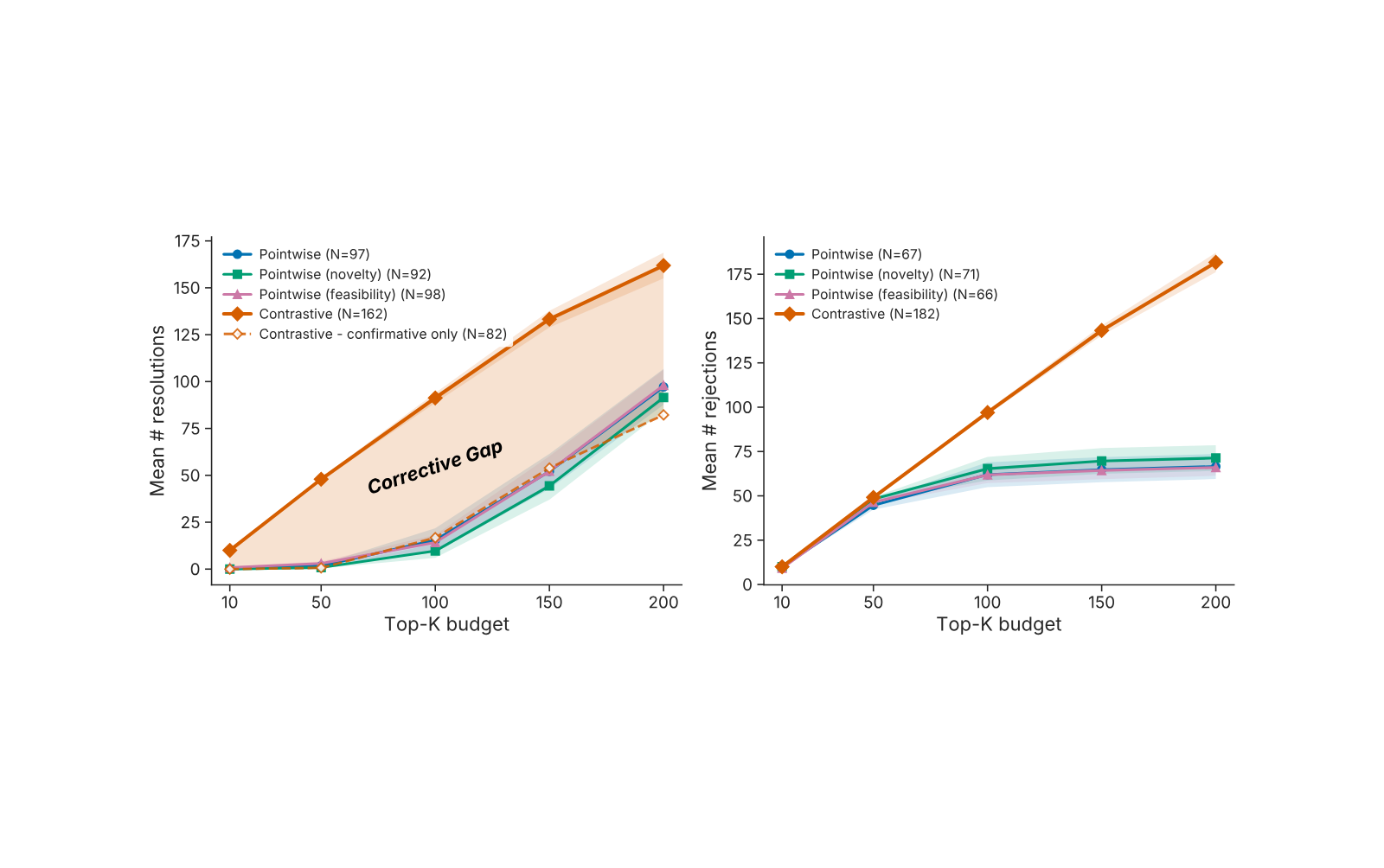
The same contrastive update that resolves a question also rules out competing alternatives, so the count of ruled-out alternatives rises with resolution. Figure 13 is a by-product of Figure 3 rather than an independent yield. Take, for example, a contrast set of three alternatives. A resolved set () leaves at most for the two remaining alternatives, so at least one of them is at most by construction, and is ruled out () unless the two split the remainder exactly evenly. The Contrastive curve counts questions with at least one ruled-out alternative, and each pointwise curve counts rejected hypotheses; bands are standard error across datasets.
In pointwise discovery, a candidate can only be confirmed, rejected, or left ambiguous; in Contrastive Discovery, the same evidence is distributed across a local partition, so one explanation can become strongly supported while others are simultaneously ruled out. Ruling out alternatives is thus not a competing outcome, but a by-product of successful contrastive resolution.
Refer to Figure 14 for decisive-unit rate and winner-switch rate. The decisive-unit rate is the fraction of top- units on which a method reached any verdict under its own gates: for pointwise, confirmed () or rejected (); for Contrastive, resolved () or at least one alternative ruled out (). It is the counterpart of the resolution rate in Figure 3 that counts a verdict in either direction for both methods: at , Full Contrastive reaches 0.91 against 0.82 for pointwise, and is higher in each of the six datasets.
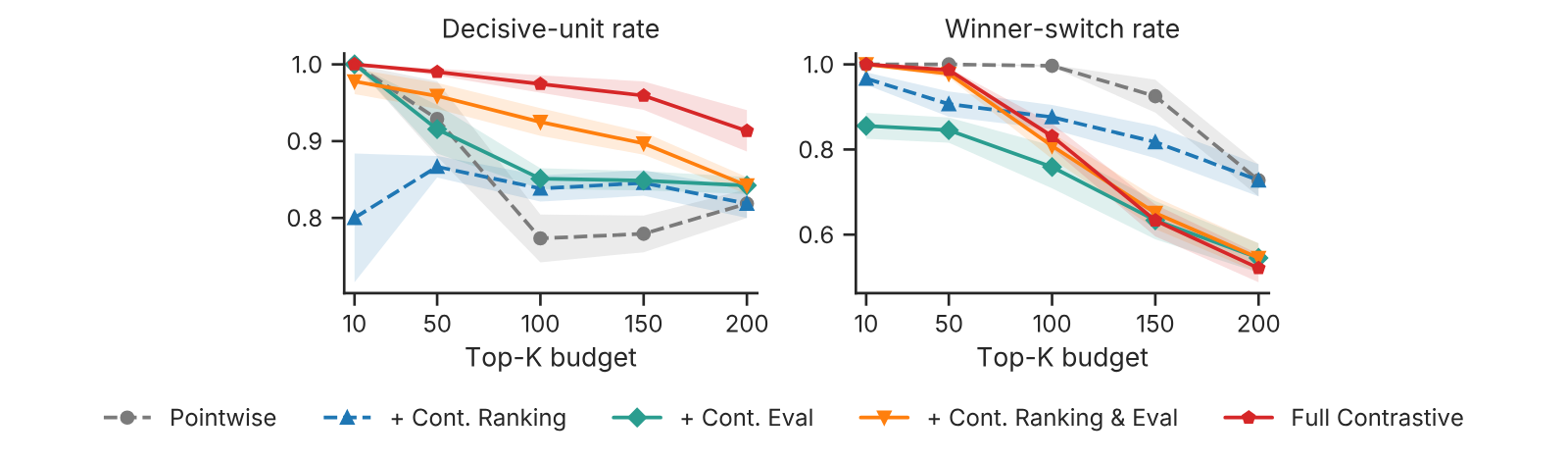
15(a) compares the Contrastive selection rules: cumulative pointwise-surprising findings when each contrast set is projected to a single member under a different rule. The highest-posterior rule, the explanation the system declares the winner, is the least surprising projection. This is expected: a resolved winner is by construction the alternative the evidence favors, so its confirmation registers little pointwise surprisal. It is the tension between resolution and surprise, not a contradiction of Appendix .
15(b)reports a structured pointwise-prompt ablation, in which the single-hypothesis generator receives a contrast-style prompt. On cumulative surprisal its curve sits visibly above the vanilla pointwise baseline; we did not run a statistical test on this difference, and the appropriate comparator on the Contrastive side is the random-projection curve of 15(a) (not the highest-prior projection), against which the variant shows no clear difference. Because it is reported on surprisal rather than on resolution, it does not bear on the headline comparison of Section 5.2; the headline comparison uses the standard pointwise baseline, and evaluating this variant on resolution is future work.
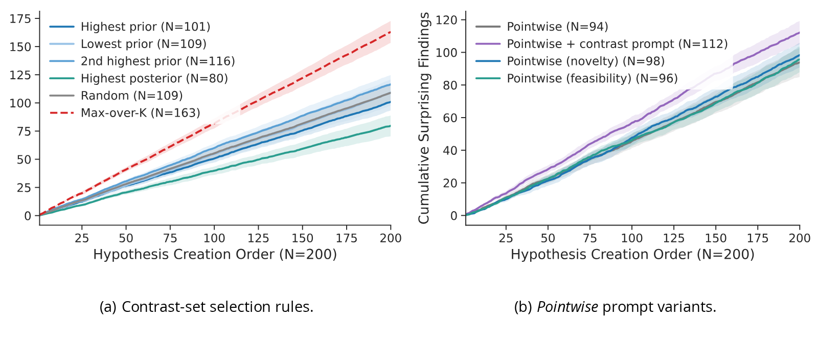
We report the hyperparameters involved in our experiments here. Refer to Tables R, , and . All settings are shared between the pointwise and Contrastive conditions except the belief-elicitation format and sample counts listed under each metric; the pointwise evidence weight is defined in Appendix . Every agent and elicitor call uses gpt-4o-2024-08-06, except where a section names another model (the cross-family elicitors of Appendix A, the cross-provider judge of Appendix C, the matcher of Appendix L, and the judge of Appendix N).
| Setting | Value |
View original table
